Why Kernels
Welcome to the 30th part of our machine learning tutorial series and the next part in our Support Vector Machine section. In this tutorial, we're going to continue talking about Kernels, mainly regarding how to actually use them now that we know we can.
As we learned before, we can utilize a Kernel to help us translate our data to a plausibly infinite number of dimensions in order to find one that has linear separability. We also learned that kernels can let us go out to these dimensions without actually paying the cost for these higher dimensions. Generally, kernels will be defined by something like:
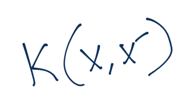
The kernel function is applied to x and x prime, and will equal the inner product of z and z prime, where the z values are from the z dimension (our new dimension space).
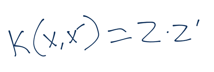
The z values are the result of some function(x), and these z values are dotted together to give us our kernel function's result.
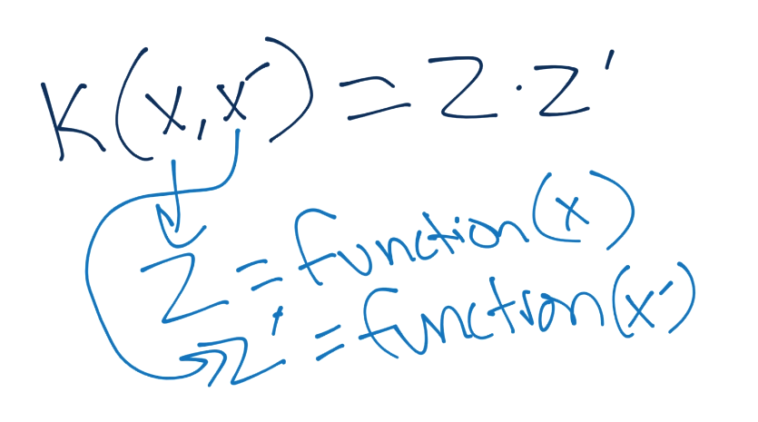
We still have yet to cover how this saves us any processing, so let's see an example. We'll start with the polynomial kernel, and compare the requirements of a polynomial kernel to simply taking our current vector and creating a 2nd order polynomial from it.

The kernel applies the same function both x and x prime, so we'd make the same thing for z prime (x prime to the second order polynomial). From there, the final step is to take the dot product of the two:
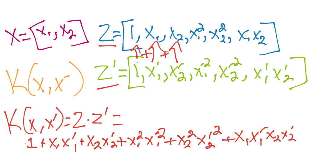
So all of that work was us manually working through a similar operation that the polynomial kernel is going to do. Luckily for us, our starting dimensions were only two! Now let's consider the polynomial kernel:

Notice right away, there are NO Z's mentioned here. This entire kernel is calculated using ONLY the x space! All you need here is to calculate using n number of dimensions and p for the power you want to use. Your equation will look something like:
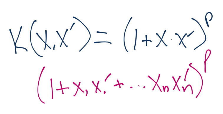
If you calculate this all out, your new vectors, which would correspond to the z-space vectors would be something like:

That said, you never need to go out that far. You simply stick with the polynomial kernel, which is going to simply return the dot product for you, without you needing to actually calculate the vectors then take a very large dot product!
There are quite a few pre-made kernels, but the only other one I will show here is the Radial Basis Function (RBF) kernel, purely since it's typically the default kernel used, and can take us to a proposed "infinite" number of dimensions
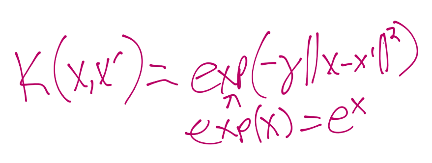
The value for gamma there is the topic of some possibly future tutorial. So there you have kernels, why you would want to use them, how to use them, and hopefully a decent depiction of how they can allow you to work with larger dimensions without paying the extremely high processing costs! In the next tutorial, we're going to talk about another solution to both non-linear data, as well as to over-fitment issues with data.
-
Practical Machine Learning Tutorial with Python Introduction
-
Regression - Intro and Data
-
Regression - Features and Labels
-
Regression - Training and Testing
-
Regression - Forecasting and Predicting
-
Pickling and Scaling
-
Regression - Theory and how it works
-
Regression - How to program the Best Fit Slope
-
Regression - How to program the Best Fit Line
-
Regression - R Squared and Coefficient of Determination Theory
-
Regression - How to Program R Squared
-
Creating Sample Data for Testing
-
Classification Intro with K Nearest Neighbors
-
Applying K Nearest Neighbors to Data
-
Euclidean Distance theory
-
Creating a K Nearest Neighbors Classifer from scratch
-
Creating a K Nearest Neighbors Classifer from scratch part 2
-
Testing our K Nearest Neighbors classifier
-
Final thoughts on K Nearest Neighbors
-
Support Vector Machine introduction
-
Vector Basics
-
Support Vector Assertions
-
Support Vector Machine Fundamentals
-
Constraint Optimization with Support Vector Machine
-
Beginning SVM from Scratch in Python
-
Support Vector Machine Optimization in Python
-
Support Vector Machine Optimization in Python part 2
-
Visualization and Predicting with our Custom SVM
-
Kernels Introduction
-
Why Kernels
-
Soft Margin Support Vector Machine
-
Kernels, Soft Margin SVM, and Quadratic Programming with Python and CVXOPT
-
Support Vector Machine Parameters
-
Machine Learning - Clustering Introduction
-
Handling Non-Numerical Data for Machine Learning
-
K-Means with Titanic Dataset
-
K-Means from Scratch in Python
-
Finishing K-Means from Scratch in Python
-
Hierarchical Clustering with Mean Shift Introduction
-
Mean Shift applied to Titanic Dataset
-
Mean Shift algorithm from scratch in Python
-
Dynamically Weighted Bandwidth for Mean Shift
-
Introduction to Neural Networks
-
Installing TensorFlow for Deep Learning - OPTIONAL
-
Introduction to Deep Learning with TensorFlow
-
Deep Learning with TensorFlow - Creating the Neural Network Model
-
Deep Learning with TensorFlow - How the Network will run
-
Deep Learning with our own Data
-
Simple Preprocessing Language Data for Deep Learning
-
Training and Testing on our Data for Deep Learning
-
10K samples compared to 1.6 million samples with Deep Learning
-
How to use CUDA and the GPU Version of Tensorflow for Deep Learning
-
Recurrent Neural Network (RNN) basics and the Long Short Term Memory (LSTM) cell
-
RNN w/ LSTM cell example in TensorFlow and Python
-
Convolutional Neural Network (CNN) basics
-
Convolutional Neural Network CNN with TensorFlow tutorial
-
TFLearn - High Level Abstraction Layer for TensorFlow Tutorial
-
Using a 3D Convolutional Neural Network on medical imaging data (CT Scans) for Kaggle
-
Classifying Cats vs Dogs with a Convolutional Neural Network on Kaggle
-
Using a neural network to solve OpenAI's CartPole balancing environment
