Regression - Intro and Data

Welcome to the introduction to the regression section of the Machine Learning with Python tutorial series. By this point, you should have Scikit-Learn already installed. If not, get it, along with Pandas and matplotlib!

Dependencies:

pip install numpy

pip install scipy

pip install scikit-learn

pip install matplotlib

pip install pandas

Along with those tutorial-wide imports, we're also going to be making use of Quandl here, which you may need to separately install, with:

pip install quandl

I will note again in the first part of the code, but the Quandl module used to be imported with an upper-case Q, but is now imported with a lower-cased q. In the video and sample codes, it is upper-cased.

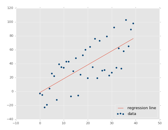
To begin, what is regression in terms of us using it with machine learning? The goal is to take continuous data, find the equation that best fits the data, and be able forecast out a specific value. With simple linear regression, you are just simply doing this by creating a best fit line:

From here, we can use the equation of that line to forecast out into the future, where the 'date' is the x-axis, what the price will be.

A popular use with regression is to predict stock prices. This is done because we are considering the fluidity of price over time, and attempting to forecast the next fluid price in the future using a continuous dataset.

Regression is a form of supervised machine learning, which is where the scientist teaches the machine by showing it features and then showing it what the correct answer is, over and over, to teach the machine. Once the machine is taught, the scientist will usually "test" the machine on some unseen data, where the scientist still knows what the correct answer is, but the machine doesn't. The machine's answers are compared to the known answers, and the machine's accuracy can be measured. If the accuracy is high enough, the scientist may consider actually employing the algorithm in the real world.

Since regression is so popularly used with stock prices, we can start there with an example. To begin, we need data. Sometimes the data is easy to acquire, and sometimes you have to go out and scrape it together, like what we did in an older tutorial series using machine learning with stock fundamentals for investing. In our case, we're able to at least start with simple stock price and volume information from Quandl. To begin, we'll start with data that grabs the stock price for Alphabet (previously Google), with the ticker of GOOGL:

import pandas as pd
import Quandl

df = Quandl.get("WIKI/GOOGL")

print(df.head())

Note: when filmed, Quandl's module was referenced with a an upper-case Q, now it is a lower-case q, so import quandl

At this point, we have:

              Open    High     Low   Close    Volume  Ex-Dividend  \
Date
2004-08-19  100.00  104.06   95.96  100.34  44659000            0
2004-08-20  101.01  109.08  100.50  108.31  22834300            0
2004-08-23  110.75  113.48  109.05  109.40  18256100            0
2004-08-24  111.24  111.60  103.57  104.87  15247300            0
2004-08-25  104.96  108.00  103.88  106.00   9188600            0

            Split Ratio  Adj. Open  Adj. High  Adj. Low  Adj. Close  \
Date
2004-08-19            1     50.000      52.03    47.980      50.170
2004-08-20            1     50.505      54.54    50.250      54.155
2004-08-23            1     55.375      56.74    54.525      54.700
2004-08-24            1     55.620      55.80    51.785      52.435
2004-08-25            1     52.480      54.00    51.940      53.000

            Adj. Volume
Date
2004-08-19     44659000
2004-08-20     22834300
2004-08-23     18256100
2004-08-24     15247300
2004-08-25      9188600 

Awesome, off to a good start, we have the data, but maybe a bit much. To reference the intro, there exists an entire machine learning category that aims to reduce the amount of input that we process. In our case, we have quite a few columns, many are redundant, a couple don't really change. We can most likely agree that having both the regular columns and adjusted columns is redundant. Adjusted columns are the most ideal ones. Regular columns here are prices on the day, but stocks have things called stock splits, where suddenly 1 share becomes something like 2 shares, thus the value of a share is halved, but the value of the company has not halved. Adjusted columns are adjusted for stock splits over time, which makes them more reliable for doing analysis.

Thus, let's go ahead and pair down our original dataframe a bit:

df = df[['Adj. Open',  'Adj. High',  'Adj. Low',  'Adj. Close', 'Adj. Volume']]

Now we just have the adjusted columns, and the volume column. A couple major points to make here. Many people talk about or hear about machine learning as if it is some sort of dark art that somehow generates value from nothing. Machine learning can highlight value if it is there, but it has to actually be there. You need meaningful data. So how do you know if you have meaningful data? My best suggestion is to just simply use your brain. Think about it. Are historical prices indicative of future prices? Some people think so, but this has been continually disproven over time. What about historical patterns? This has a bit more merit when taken to the extremes (which machine learning can help with), but is overall fairly weak. What about the relationship between price changes and volume over time, along with historical patterns? Probably a bit better. So, as you can already see, it is not the case that the more data the merrier, but we instead want to use useful data. At the same time, raw data sometimes should be transformed.

Consider daily volatility, such as with the high minus low % change? How about daily percent change? Would you consider data that is simply the Open, High, Low, Close or data that is the Close, Spread/Volatility, %change daily to be better? I would expect the latter to be more ideal. The former is all very similar data points. The latter is created based on the identical data from the former, but it brings far more valuable information to the table.

Thus, not all of the data you have is useful, and sometimes you need to do further manipulation on your data to make it even more valuable before feeding it through a machine learning algorithm. Let's go ahead and transform our data next:

df['HL_PCT'] = (df['Adj. High'] - df['Adj. Low']) / df['Adj. Close'] * 100.0

I went ahead and recorded the video version of this, not realizing my stake that it was high minus low divided by close. I meant to do High - Low, divided by the low. Feel free to fix that if you like.

This creates a new column that is the % spread based on the closing price, which is our crude measure of volatility. Next, we'll do daily percent change:

df['PCT_change'] = (df['Adj. Close'] - df['Adj. Open']) / df['Adj. Open'] * 100.0

Now we will define a new dataframe as:

df = df[['Adj. Close', 'HL_PCT', 'PCT_change', 'Adj. Volume']]
print(df.head())

            Adj. Close    HL_PCT  PCT_change  Adj. Volume
Date
2004-08-19      50.170  8.072553    0.340000     44659000
2004-08-20      54.155  7.921706    7.227007     22834300
2004-08-23      54.700  4.049360   -1.218962     18256100
2004-08-24      52.435  7.657099   -5.726357     15247300
2004-08-25      53.000  3.886792    0.990854      9188600

The next tutorial: Regression - Features and Labels