Visualization and Predicting with our Custom SVM
Welcome to the 28th part of our machine learning tutorial series and the next part in our Support Vector Machine section. In this tutorial, we're going to finish off our basic Support Vector Machine from scratch and see it visually as well as make a prediction!
Our code up to this point:
import matplotlib.pyplot as plt
from matplotlib import style
import numpy as np
style.use('ggplot')

class Support_Vector_Machine:
    def __init__(self, visualization=True):
        self.visualization = visualization
        self.colors = {1:'r',-1:'b'}
        if self.visualization:
            self.fig = plt.figure()
            self.ax = self.fig.add_subplot(1,1,1)
    # train
    def fit(self, data):
        self.data = data
        # { ||w||: [w,b] }
        opt_dict = {}

        transforms = [[1,1],
                      [-1,1],
                      [-1,-1],
                      [1,-1]]

        all_data = []
        for yi in self.data:
            for featureset in self.data[yi]:
                for feature in featureset:
                    all_data.append(feature)

        self.max_feature_value = max(all_data)
        self.min_feature_value = min(all_data)
        all_data = None

        # support vectors yi(xi.w+b) = 1


        step_sizes = [self.max_feature_value * 0.1,
                      self.max_feature_value * 0.01,
                      # point of expense:
                      self.max_feature_value * 0.001,]


        # extremely expensive
        b_range_multiple = 5
        # we dont need to take as small of steps
        # with b as we do w
        b_multiple = 5
        latest_optimum = self.max_feature_value*10

        for step in step_sizes:
            w = np.array([latest_optimum,latest_optimum])
            # we can do this because convex
            optimized = False
            while not optimized:
                for b in np.arange(-1*(self.max_feature_value*b_range_multiple),
                                   self.max_feature_value*b_range_multiple,
                                   step*b_multiple):
                    for transformation in transforms:
                        w_t = w*transformation
                        found_option = True
                        # weakest link in the SVM fundamentally
                        # SMO attempts to fix this a bit
                        # yi(xi.w+b) >= 1
                        #
                        # #### add a break here later..
                        for i in self.data:
                            for xi in self.data[i]:
                                yi=i
                                if not yi*(np.dot(w_t,xi)+b) >= 1:
                                    found_option = False

                        if found_option:
                            opt_dict[np.linalg.norm(w_t)] = [w_t,b]

                if w[0] < 0:
                    optimized = True
                    print('Optimized a step.')
                else:
                    w = w - step

            norms = sorted([n for n in opt_dict])
            #||w|| : [w,b]
            opt_choice = opt_dict[norms[0]]
            self.w = opt_choice[0]
            self.b = opt_choice[1]
            latest_optimum = opt_choice[0][0]+step*2


    def predict(self,features):
        # sign( x.w+b )
        classification = np.sign(np.dot(np.array(features),self.w)+self.b)
        return classification


data_dict = {-1:np.array([[1,7],
                          [2,8],
                          [3,8],]),

             1:np.array([[5,1],
                         [6,-1],
                         [7,3],])}
We already have a predict method, since that is a fairly easy step, but now we're going to add a bit to it to handle for visualizing the predictions:
    def predict(self,features):
        # classifiction is just:
        # sign(xi.w+b)
        classification = np.sign(np.dot(np.array(features),self.w)+self.b)
        # if the classification isn't zero, and we have visualization on, we graph
        if classification != 0 and self.visualization:
            self.ax.scatter(features[0],features[1],s=200,marker='*', c=self.colors[classification])
        else:
            print('featureset',features,'is on the decision boundary')
        return classification
Above, all we've added is handling to also visualize the prediction if we have one. We're just going to do one at a time, but you could augment the code to do many at once like scikit-learn does.
Next, let's begin building our visualize method:
    def visualize(self):
        #scattering known featuresets.
        [[self.ax.scatter(x[0],x[1],s=100,color=self.colors[i]) for x in data_dict[i]] for i in data_dict]
All that one liner is doing is going through our data and graphing it along with its associated color. See the video if you want to see it more broken down.
Next, we want to graph our hyperplanes for the positive and negative support vectors, along with the decision boundary. In order to do this, we need at least two points for each to create a "line" which will be our hyperplane.
Once we know what w and b are, we can use algebra to create a function that will return to us the value needed for our second feature (x2) to make the line:
        def hyperplane(x,w,b,v):
            # v = (w.x+b)
            return (-w[0]*x-b+v) / w[1]
Next up, we create some variables to house various data that we're going to reference:
        datarange = (self.min_feature_value*0.9,self.max_feature_value*1.1)
        hyp_x_min = datarange[0]
        hyp_x_max = datarange[1]
Our main goal here is to establish to what values we want to actually draw our hyperplanes.
Now, let's graph our positive support vector hyperplane:
        # w.x + b = 1
        # pos sv hyperplane
        psv1 = hyperplane(hyp_x_min, self.w, self.b, 1)
        psv2 = hyperplane(hyp_x_max, self.w, self.b, 1)
        self.ax.plot([hyp_x_min,hyp_x_max], [psv1,psv2], "k")
Simple e nough, we get the data for the first and second x2 values, then we graph them. Now we'll do the next two hyperplanes:
        # w.x + b = -1
        # negative sv hyperplane
        nsv1 = hyperplane(hyp_x_min, self.w, self.b, -1)
        nsv2 = hyperplane(hyp_x_max, self.w, self.b, -1)
        self.ax.plot([hyp_x_min,hyp_x_max], [nsv1,nsv2], "k")

        # w.x + b = 0
        # decision
        db1 = hyperplane(hyp_x_min, self.w, self.b, 0)
        db2 = hyperplane(hyp_x_max, self.w, self.b, 0)
        self.ax.plot([hyp_x_min,hyp_x_max], [db1,db2], "g--")

        plt.show()
Now, adding some code at the bottom for training, predicting, and visualizing:
import matplotlib.pyplot as plt
from matplotlib import style
import numpy as np
style.use('ggplot')
class Support_Vector_Machine:
def __init__(self, visualization=True):
self.visualization = visualization
self.colors = {1:'r',-1:'b'}
if self.visualization:
self.fig = plt.figure()
self.ax = self.fig.add_subplot(1,1,1)
# train
def fit(self, data):
self.data = data
# { ||w||: [w,b] }
opt_dict = {}
transforms = [[1,1],
[-1,1],
[-1,-1],
[1,-1]]
all_data = []
for yi in self.data:
for featureset in self.data[yi]:
for feature in featureset:
all_data.append(feature)
self.max_feature_value = max(all_data)
self.min_feature_value = min(all_data)
all_data = None
# support vectors yi(xi.w+b) = 1
step_sizes = [self.max_feature_value * 0.1,
self.max_feature_value * 0.01,
# point of expense:
self.max_feature_value * 0.001,
]
# extremely expensive
b_range_multiple = 2
# we dont need to take as small of steps
# with b as we do w
b_multiple = 5
latest_optimum = self.max_feature_value*10
for step in step_sizes:
w = np.array([latest_optimum,latest_optimum])
# we can do this because convex
optimized = False
while not optimized:
for b in np.arange(-1*(self.max_feature_value*b_range_multiple),
self.max_feature_value*b_range_multiple,
step*b_multiple):
for transformation in transforms:
w_t = w*transformation
found_option = True
# weakest link in the SVM fundamentally
# SMO attempts to fix this a bit
# yi(xi.w+b) >= 1
#
# #### add a break here later..
for i in self.data:
for xi in self.data[i]:
yi=i
if not yi*(np.dot(w_t,xi)+b) >= 1:
found_option = False
#print(xi,':',yi*(np.dot(w_t,xi)+b))
if found_option:
opt_dict[np.linalg.norm(w_t)] = [w_t,b]
if w[0] < 0:
optimized = True
print('Optimized a step.')
else:
w = w - step
norms = sorted([n for n in opt_dict])
#||w|| : [w,b]
opt_choice = opt_dict[norms[0]]
self.w = opt_choice[0]
self.b = opt_choice[1]
latest_optimum = opt_choice[0][0]+step*2
for i in self.data:
for xi in self.data[i]:
yi=i
print(xi,':',yi*(np.dot(self.w,xi)+self.b))
def predict(self,features):
# sign( x.w+b )
classification = np.sign(np.dot(np.array(features),self.w)+self.b)
if classification !=0 and self.visualization:
self.ax.scatter(features[0], features[1], s=200, marker='*', c=self.colors[classification])
return classification
def visualize(self):
[[self.ax.scatter(x[0],x[1],s=100,color=self.colors[i]) for x in data_dict[i]] for i in data_dict]
# hyperplane = x.w+b
# v = x.w+b
# psv = 1
# nsv = -1
# dec = 0
def hyperplane(x,w,b,v):
return (-w[0]*x-b+v) / w[1]
datarange = (self.min_feature_value*0.9,self.max_feature_value*1.1)
hyp_x_min = datarange[0]
hyp_x_max = datarange[1]
# (w.x+b) = 1
# positive support vector hyperplane
psv1 = hyperplane(hyp_x_min, self.w, self.b, 1)
psv2 = hyperplane(hyp_x_max, self.w, self.b, 1)
self.ax.plot([hyp_x_min,hyp_x_max],[psv1,psv2], 'k')
# (w.x+b) = -1
# negative support vector hyperplane
nsv1 = hyperplane(hyp_x_min, self.w, self.b, -1)
nsv2 = hyperplane(hyp_x_max, self.w, self.b, -1)
self.ax.plot([hyp_x_min,hyp_x_max],[nsv1,nsv2], 'k')
# (w.x+b) = 0
# positive support vector hyperplane
db1 = hyperplane(hyp_x_min, self.w, self.b, 0)
db2 = hyperplane(hyp_x_max, self.w, self.b, 0)
self.ax.plot([hyp_x_min,hyp_x_max],[db1,db2], 'y--')
plt.show()
data_dict = {-1:np.array([[1,7],
[2,8],
[3,8],]),
1:np.array([[5,1],
[6,-1],
[7,3],])}
svm = Support_Vector_Machine()
svm.fit(data=data_dict)
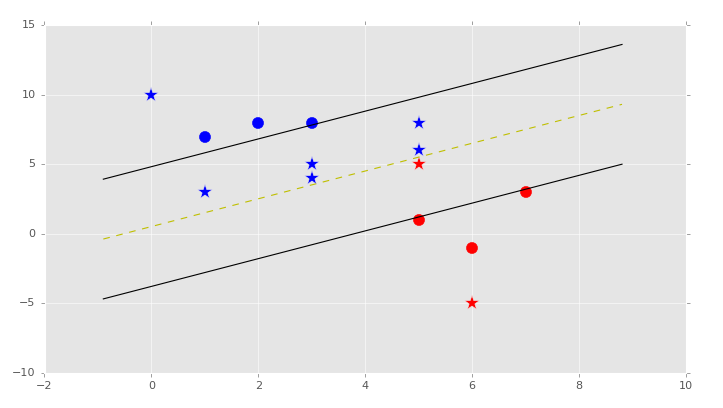
predict_us = [[0,10],
[1,3],
[3,4],
[3,5],
[5,5],
[5,6],
[6,-5],
[5,8]]
for p in predict_us:
svm.predict(p)
svm.visualize()
Our result:
-
Practical Machine Learning Tutorial with Python Introduction
-
Regression - Intro and Data
-
Regression - Features and Labels
-
Regression - Training and Testing
-
Regression - Forecasting and Predicting
-
Pickling and Scaling
-
Regression - Theory and how it works
-
Regression - How to program the Best Fit Slope
-
Regression - How to program the Best Fit Line
-
Regression - R Squared and Coefficient of Determination Theory
-
Regression - How to Program R Squared
-
Creating Sample Data for Testing
-
Classification Intro with K Nearest Neighbors
-
Applying K Nearest Neighbors to Data
-
Euclidean Distance theory
-
Creating a K Nearest Neighbors Classifer from scratch
-
Creating a K Nearest Neighbors Classifer from scratch part 2
-
Testing our K Nearest Neighbors classifier
-
Final thoughts on K Nearest Neighbors
-
Support Vector Machine introduction
-
Vector Basics
-
Support Vector Assertions
-
Support Vector Machine Fundamentals
-
Constraint Optimization with Support Vector Machine
-
Beginning SVM from Scratch in Python
-
Support Vector Machine Optimization in Python
-
Support Vector Machine Optimization in Python part 2
-
Visualization and Predicting with our Custom SVM
-
Kernels Introduction
-
Why Kernels
-
Soft Margin Support Vector Machine
-
Kernels, Soft Margin SVM, and Quadratic Programming with Python and CVXOPT
-
Support Vector Machine Parameters
-
Machine Learning - Clustering Introduction
-
Handling Non-Numerical Data for Machine Learning
-
K-Means with Titanic Dataset
-
K-Means from Scratch in Python
-
Finishing K-Means from Scratch in Python
-
Hierarchical Clustering with Mean Shift Introduction
-
Mean Shift applied to Titanic Dataset
-
Mean Shift algorithm from scratch in Python
-
Dynamically Weighted Bandwidth for Mean Shift
-
Introduction to Neural Networks
-
Installing TensorFlow for Deep Learning - OPTIONAL
-
Introduction to Deep Learning with TensorFlow
-
Deep Learning with TensorFlow - Creating the Neural Network Model
-
Deep Learning with TensorFlow - How the Network will run
-
Deep Learning with our own Data
-
Simple Preprocessing Language Data for Deep Learning
-
Training and Testing on our Data for Deep Learning
-
10K samples compared to 1.6 million samples with Deep Learning
-
How to use CUDA and the GPU Version of Tensorflow for Deep Learning
-
Recurrent Neural Network (RNN) basics and the Long Short Term Memory (LSTM) cell
-
RNN w/ LSTM cell example in TensorFlow and Python
-
Convolutional Neural Network (CNN) basics
-
Convolutional Neural Network CNN with TensorFlow tutorial
-
TFLearn - High Level Abstraction Layer for TensorFlow Tutorial
-
Using a 3D Convolutional Neural Network on medical imaging data (CT Scans) for Kaggle
-
Classifying Cats vs Dogs with a Convolutional Neural Network on Kaggle
-
Using a neural network to solve OpenAI's CartPole balancing environment
