Support Vector Machine introduction
Welcome to the 20th part of our machine learning tutorial series. We are now going to dive into another form of supervised machine learning and classification: Support Vector Machines.
The Support Vector Machine, created by Vladimir Vapnik in the 60s, but pretty much overlooked until the 90s is still one of most popular machine learning classifiers.
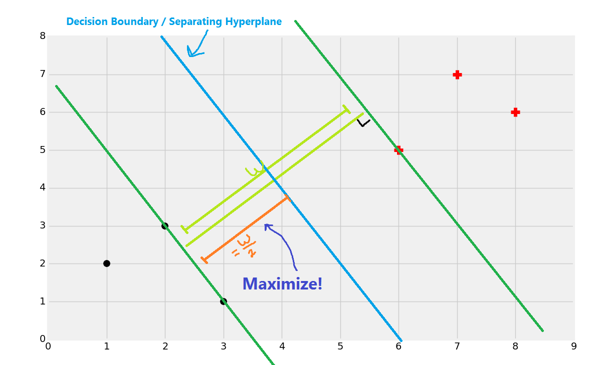
The objective of the Support Vector Machine is to find the best splitting boundary between data. In two dimensional space, you can think of this like the best fit line that divides your dataset. With a Support Vector Machine, we're dealing in vector space, thus the separating line is actually a separating hyperplane. The best separating hyperplane is defined as the hyperplane that contains the "widest" margin between support vectors. The hyperplane may also be referred to as a decision boundary. The easiest way to convey this is through images:
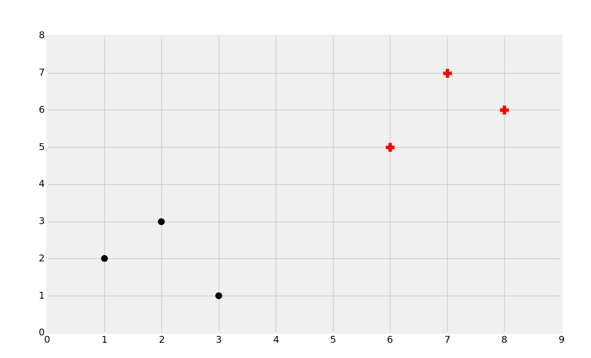
We will start with the above data. We noted in the past that the most common intuition is that you would classify a new data point based on what it is closest to or the proximity, which is what the K Nearest Neighbors algorithm does for us. The main issue with this objective is that, per datapoint, you have to compare it to every single datapoint to get the distances, thus the algorithm just doesn't scale well, despite being fairly reliable accuracy-wise. What the Support Vector Machine aims to do is, one time, generate the "best fit" line (but actually a plane, and even more specifically a hyperplane!) that best divides the data. Once this hyperplane is discovered, we refer to it as a decision boundary. We do this, because, this is the boundary between being one class or another. Once we calculate this decision boundary, we never need to do it again, unless of course we are re-training the dataset. Thus, this algorithm is going to scale, unlike the KNN classifier.
The curiosity is, of course, how do we actually figure out that best dividing hyperplane? Well, we can eye-ball this.
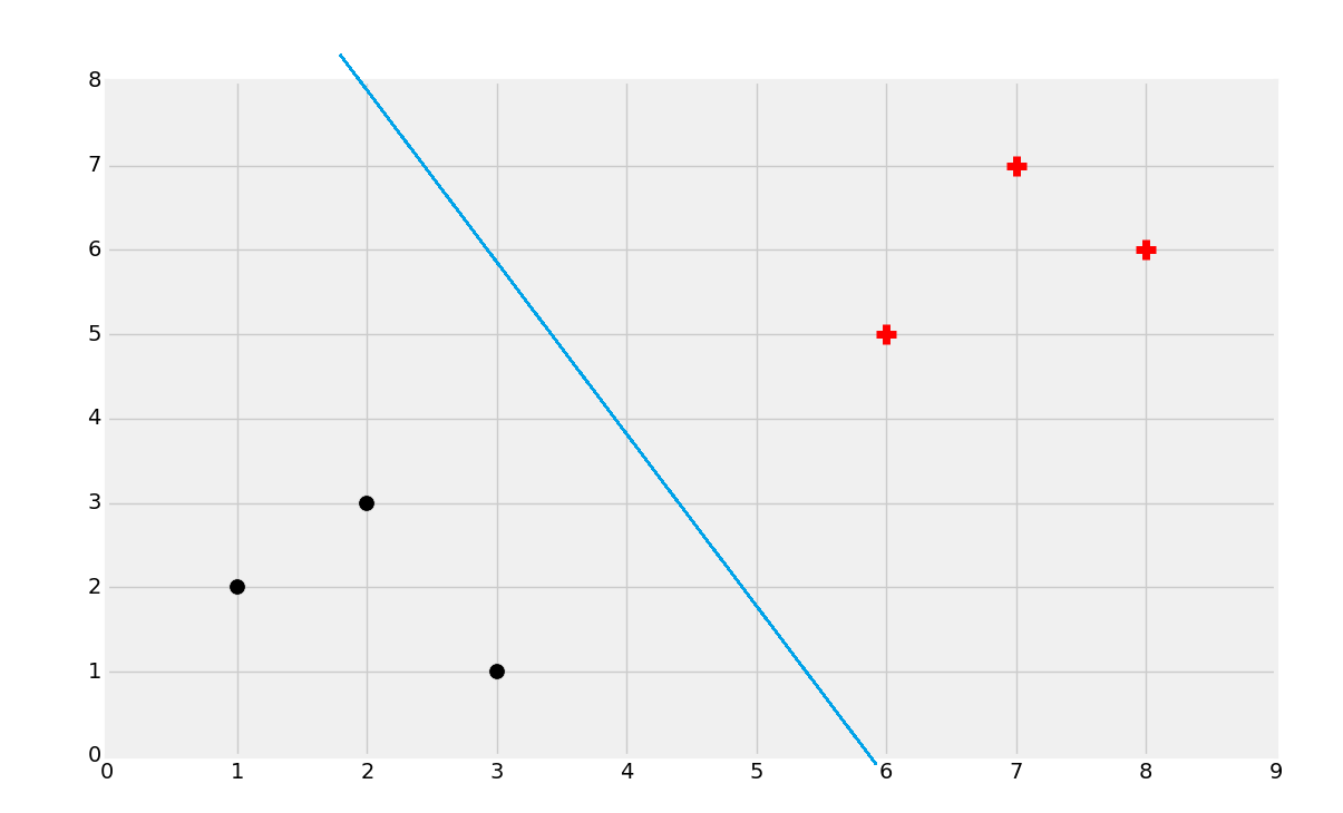
That's probably about right, but, how do we find that? Well, first you find the support vectors:
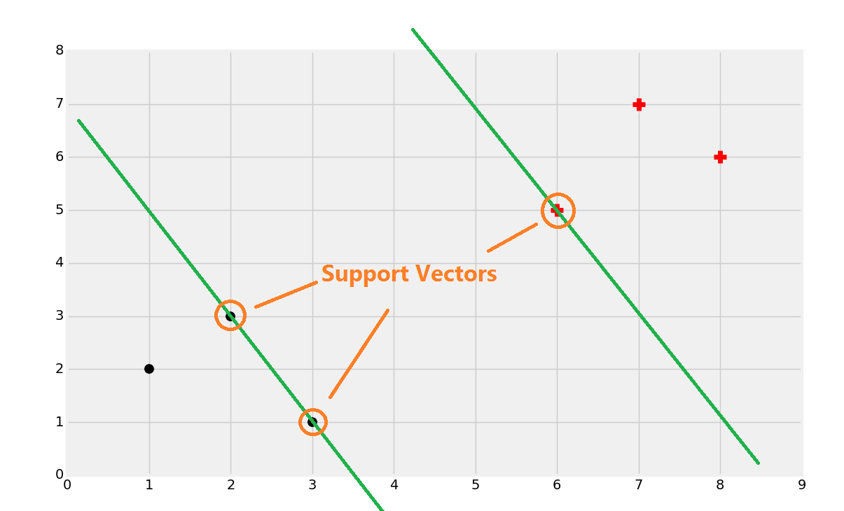
Once you find the support vectors, you want to create lines that are maximally separated between each other. From here, we can easily find the decision boundary by taking the total width:
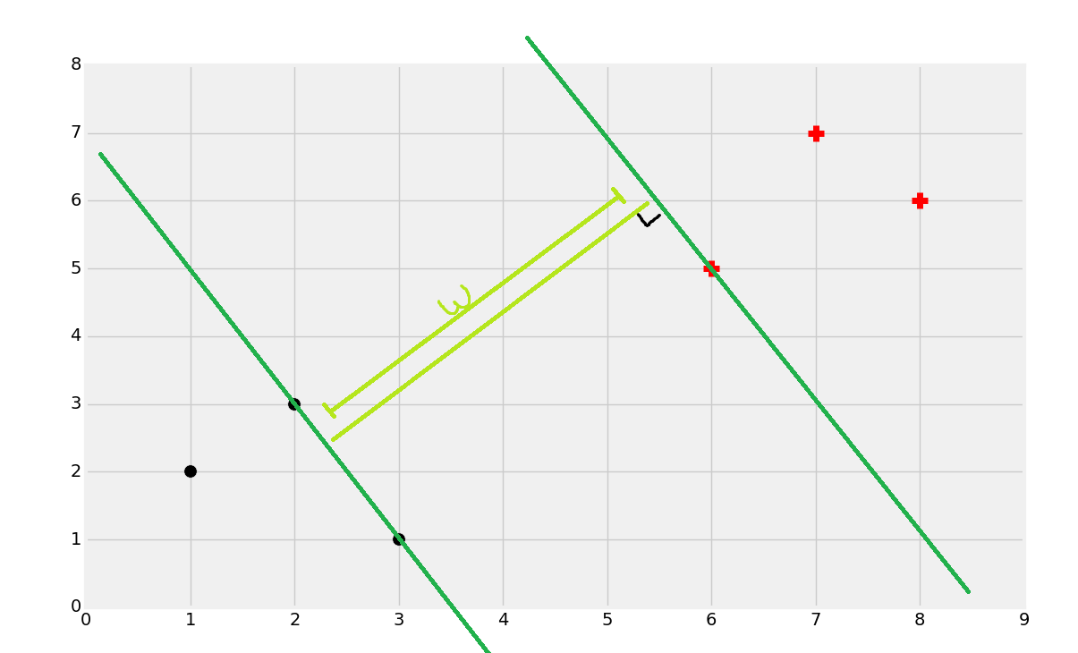
Dividing by 2:
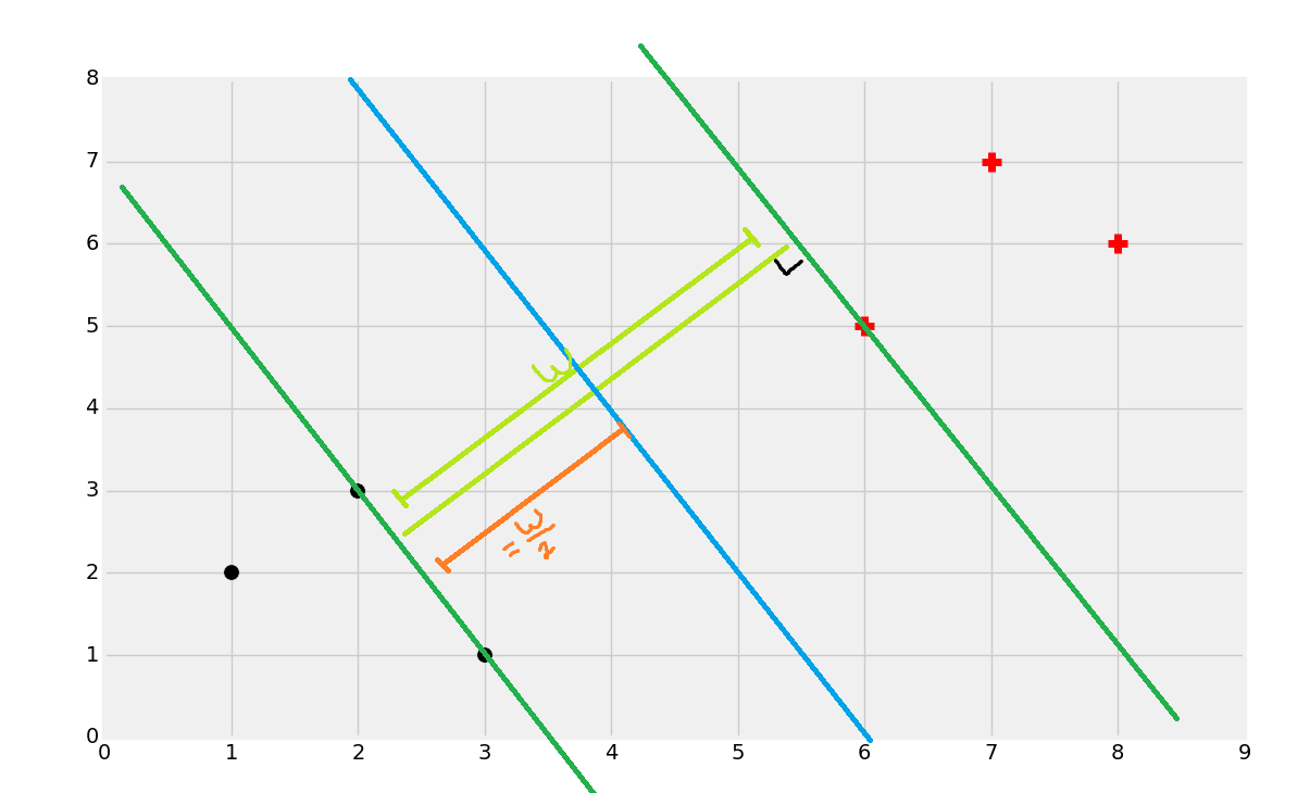
And you've got your boundary:
Now if a point is to the left of the decision boundary/separating hyperplane, then we say it's a black dot class. If it is to the right, then it is a red plus sign class.
It is worth noting, of course, that this method of learning is only going to work natively on linearly-separable data. If you have data like:
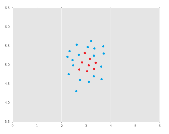
Can you create a separating hyperplane here? No. Is all hope lost? I'll let you ponder that question as we dive into an example with the Support Vector Machine. Here's a really great reason why working with Scikit-Learn is lovely. Remember the code we used with Sklearn to do K Nearest Neighbors? Here it is:
import numpy as np
from sklearn import preprocessing, cross_validation, neighbors
import pandas as pd

df = pd.read_csv('breast-cancer-wisconsin.data.txt')
df.replace('?',-99999, inplace=True)
df.drop(['id'], 1, inplace=True)

X = np.array(df.drop(['class'], 1))
y = np.array(df['class'])

X_train, X_test, y_train, y_test = cross_validation.train_test_split(X, y, test_size=0.2)

clf = neighbors.KNeighborsClassifier()


clf.fit(X_train, y_train)
confidence = clf.score(X_test, y_test)
print(confidence)

example_measures = np.array([[4,2,1,1,1,2,3,2,1]])
example_measures = example_measures.reshape(len(example_measures), -1)
prediction = clf.predict(example_measures)
print(prediction)
We need to make only two simple changes here. The first is to import svm from sklearn, and the second is just to use the Support Vector Classifier, which is just svm.SVC. With our changes now:
import numpy as np
from sklearn import preprocessing, cross_validation, neighbors, svm
import pandas as pd

df = pd.read_csv('breast-cancer-wisconsin.data.txt')
df.replace('?',-99999, inplace=True)
df.drop(['id'], 1, inplace=True)

X = np.array(df.drop(['class'], 1))
y = np.array(df['class'])

X_train, X_test, y_train, y_test = cross_validation.train_test_split(X, y, test_size=0.2)

clf = svm.SVC()

clf.fit(X_train, y_train)
confidence = clf.score(X_test, y_test)
print(confidence)

example_measures = np.array([[4,2,1,1,1,2,3,2,1]])
example_measures = example_measures.reshape(len(example_measures), -1)
prediction = clf.predict(example_measures)
print(prediction)
For me, my output was:
0.978571428571
[2]
Depending on your random sample, you should get something between 94 and 99%, averaging around 97% again. Also, timing the operation, recall that I got 0.044 seconds to execute the KNN code via Scikit-Learn. With the svm.SVC, execution time was a mere 0.00951, which is 4.6x faster on even this very small dataset.
So we can agree that the Support Vector Machine appears to get the same accuracy in this case, only at a much faster pace. Note that if we comment out the drop id column part, accuracy goes back down into the 60s. The Support Vector Machine, in general, handles pointless data better than the K Nearest Neighbors algorithm, and definitely will handle outliers better, but, in this example, the meaningless data is still very misleading for us. We are using the default parameters, however. Looking at the Documentation for the Support Vector Classification, there sure are quite a few parameters here that we have no idea what they're doing. In the coming tutorials, we're going to hop in the deep end to pull apart the Support Vector Machine algorithm so we can actually understand what all these parameters mean and how they affect things. While we're breaking things down, start thinking about: How to handle non-linearly seperable data and datasets with more than two classes (since and SVM is a binary classifier, in the sense that it draws a line to divide two groups).
There exists 3 quiz/question(s) for this tutorial. for access to these, video downloads, and no ads.
-
Practical Machine Learning Tutorial with Python Introduction
-
Regression - Intro and Data
-
Regression - Features and Labels
-
Regression - Training and Testing
-
Regression - Forecasting and Predicting
-
Pickling and Scaling
-
Regression - Theory and how it works
-
Regression - How to program the Best Fit Slope
-
Regression - How to program the Best Fit Line
-
Regression - R Squared and Coefficient of Determination Theory
-
Regression - How to Program R Squared
-
Creating Sample Data for Testing
-
Classification Intro with K Nearest Neighbors
-
Applying K Nearest Neighbors to Data
-
Euclidean Distance theory
-
Creating a K Nearest Neighbors Classifer from scratch
-
Creating a K Nearest Neighbors Classifer from scratch part 2
-
Testing our K Nearest Neighbors classifier
-
Final thoughts on K Nearest Neighbors
-
Support Vector Machine introduction
-
Vector Basics
-
Support Vector Assertions
-
Support Vector Machine Fundamentals
-
Constraint Optimization with Support Vector Machine
-
Beginning SVM from Scratch in Python
-
Support Vector Machine Optimization in Python
-
Support Vector Machine Optimization in Python part 2
-
Visualization and Predicting with our Custom SVM
-
Kernels Introduction
-
Why Kernels
-
Soft Margin Support Vector Machine
-
Kernels, Soft Margin SVM, and Quadratic Programming with Python and CVXOPT
-
Support Vector Machine Parameters
-
Machine Learning - Clustering Introduction
-
Handling Non-Numerical Data for Machine Learning
-
K-Means with Titanic Dataset
-
K-Means from Scratch in Python
-
Finishing K-Means from Scratch in Python
-
Hierarchical Clustering with Mean Shift Introduction
-
Mean Shift applied to Titanic Dataset
-
Mean Shift algorithm from scratch in Python
-
Dynamically Weighted Bandwidth for Mean Shift
-
Introduction to Neural Networks
-
Installing TensorFlow for Deep Learning - OPTIONAL
-
Introduction to Deep Learning with TensorFlow
-
Deep Learning with TensorFlow - Creating the Neural Network Model
-
Deep Learning with TensorFlow - How the Network will run
-
Deep Learning with our own Data
-
Simple Preprocessing Language Data for Deep Learning
-
Training and Testing on our Data for Deep Learning
-
10K samples compared to 1.6 million samples with Deep Learning
-
How to use CUDA and the GPU Version of Tensorflow for Deep Learning
-
Recurrent Neural Network (RNN) basics and the Long Short Term Memory (LSTM) cell
-
RNN w/ LSTM cell example in TensorFlow and Python
-
Convolutional Neural Network (CNN) basics
-
Convolutional Neural Network CNN with TensorFlow tutorial
-
TFLearn - High Level Abstraction Layer for TensorFlow Tutorial
-
Using a 3D Convolutional Neural Network on medical imaging data (CT Scans) for Kaggle
-
Classifying Cats vs Dogs with a Convolutional Neural Network on Kaggle
-
Using a neural network to solve OpenAI's CartPole balancing environment
