Mean Shift algorithm from scratch in Python

Welcome to the 41st part of our machine learning tutorial series, and another tutorial within the topic of Clustering..

In this tutorial, we begin building our own mean shift algorithm from scratch. To begin, we will start with some code from part 37 of this series, which was when we began building our custom K Means algorithm. I will add one more cluster/group to the original data. Feel free to add the new data or leave it the same as it was.

import matplotlib.pyplot as plt
from matplotlib import style
style.use('ggplot')
import numpy as np

X = np.array([[1, 2],
              [1.5, 1.8],
              [5, 8 ],
              [8, 8],
              [1, 0.6],
              [9,11],
              [8,2],
              [10,2],
              [9,3],])

plt.scatter(X[:,0], X[:,1], s=150)
plt.show()

colors = 10*["g","r","c","b","k"]

If ran, the code generates:

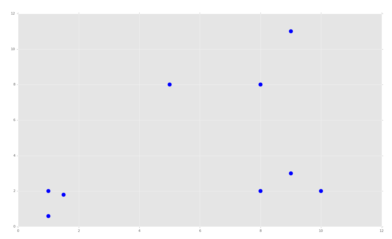
Just like in the K Means part, this creates obvious groups. With K Means, we even told the machine that we wanted 'k' clusters (2). With Mean Shift, we're expecting that the machine just figures that out on its own, and, for us, we're expecting three groups with the code above.

We will begin our Mean Shift class:

class Mean_Shift:
    def __init__(self, radius=4):
        self.radius = radius

We will start with a radius of 4, since we can estimate with our dataset that a radius of four makes sense. That's all we need for now in the initialization method. Moving on to the fit method:

    def fit(self, data):
        centroids = {}

        for i in range(len(data)):
            centroids[i] = data[i]

Here, we begin with creating starting centroids. Recall the method for Mean Shift is:

1. Make all datapoints centroids
2. Take mean of all featuresets within centroid's radius, setting this mean as new centroid.
3. Repeat step #2 until convergence.

So far we have done step 1. Now we need to repeat step 2 until convergence!

        while True:
            new_centroids = []
            for i in centroids:
                in_bandwidth = []
                centroid = centroids[i]
                for featureset in data:
                    if np.linalg.norm(featureset-centroid) < self.radius:
                        in_bandwidth.append(featureset)

                new_centroid = np.average(in_bandwidth,axis=0)
                new_centroids.append(tuple(new_centroid))

            uniques = sorted(list(set(new_centroids)))

Here, we begin iterating through each centroid, and finding all featuresets in range. From there, we are taking the average, and setting that average as the "new centroid." Finally, we're creating a uniques variable, which tracks the sorted list of all known centroids. We use set here since there may be duplicates, and duplicate centroids are really just the same centroid.

To conclude the fit method:

            prev_centroids = dict(centroids)

            centroids = {}
            for i in range(len(uniques)):
                centroids[i] = np.array(uniques[i])

            optimized = True

            for i in centroids:
                if not np.array_equal(centroids[i], prev_centroids[i]):
                    optimized = False
                if not optimized:
                    break
                
            if optimized:
                break

        self.centroids = centroids

Here we note the previous centroids, before we begin to reset "current" or "new" centroids by setting them as the uniques. Finally, we compare the previous centroids to the new ones, and measure movement. If any of the centroids have moved, then we're not content that we've got full convergence and optimization, and we want to go ahead and run another cycle. If we are optimized, great, we break, and then finally set the centroids attribute to the final centroids we came up with.

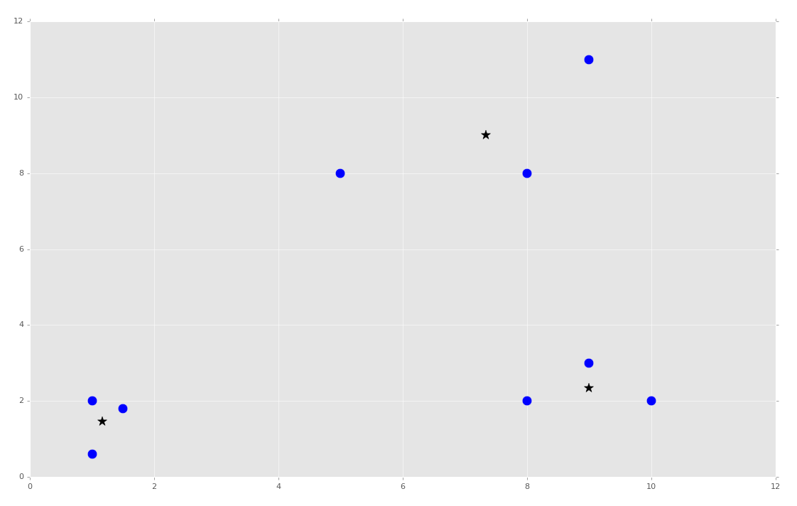
We can now wrap up this first part, and the class, adding the following:

clf = Mean_Shift()
clf.fit(X)

centroids = clf.centroids

plt.scatter(X[:,0], X[:,1], s=150)

for c in centroids:
    plt.scatter(centroids[c][0], centroids[c][1], color='k', marker='*', s=150)

plt.show()

Full code up to this point:

import matplotlib.pyplot as plt
from matplotlib import style
style.use('ggplot')
import numpy as np

X = np.array([[1, 2],
              [1.5, 1.8],
              [5, 8 ],
              [8, 8],
              [1, 0.6],
              [9,11],
              [8,2],
              [10,2],
              [9,3],])

##plt.scatter(X[:,0], X[:,1], s=150)
##plt.show()

colors = 10*["g","r","c","b","k"]

class Mean_Shift:
    def __init__(self, radius=4):
        self.radius = radius

    def fit(self, data):
        centroids = {}

        for i in range(len(data)):
            centroids[i] = data[i]
        
        while True:
            new_centroids = []
            for i in centroids:
                in_bandwidth = []
                centroid = centroids[i]
                for featureset in data:
                    if np.linalg.norm(featureset-centroid) < self.radius:
                        in_bandwidth.append(featureset)

                new_centroid = np.average(in_bandwidth,axis=0)
                new_centroids.append(tuple(new_centroid))

            uniques = sorted(list(set(new_centroids)))

            prev_centroids = dict(centroids)

            centroids = {}
            for i in range(len(uniques)):
                centroids[i] = np.array(uniques[i])

            optimized = True

            for i in centroids:
                if not np.array_equal(centroids[i], prev_centroids[i]):
                    optimized = False
                if not optimized:
                    break
                
            if optimized:
                break

        self.centroids = centroids



clf = Mean_Shift()
clf.fit(X)

centroids = clf.centroids

plt.scatter(X[:,0], X[:,1], s=150)

for c in centroids:
    plt.scatter(centroids[c][0], centroids[c][1], color='k', marker='*', s=150)

plt.show()

At this point, we've got the centroids we need, and we're feeling pretty smart. From here, all we need to do is calculate the Euclidean distances, and we have our clusters and classifications! Predictions are easy from there! There's just one problem: The radius

We've basically hard-coded the radius. I did it by looking at the dataset and deciding 4 was a good number. It's not dynamic at all, and this is supposed to be unsupervised machine learning. Imagine if we had 50 dimensions? It wouldn't be so simple. Can a machine look at the dataset and come up with something decent? We'll cover that as well as predictions in the next tutorial.

The next tutorial: Dynamically Weighted Bandwidth for Mean Shift