Pickling and Scaling
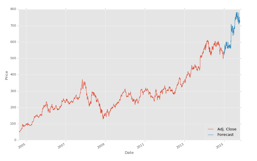
In the previous Machine Learning with Python tutorial we finished up making a forecast of stock prices using regression, and then visualizing the forecast with Matplotlib. In this tutorial, we'll talk about some next steps.
I remember the first time that I was trying to learn about machine learning, and most examples were only covering up to the training and testing part, totally skipping the prediction part. Of the tutorials that did the training, testing, and predicting part, I did not find a single one that explained saving the algorithm. With examples, data is generally pretty small overall, so the training, testing, and prediction process is relatively fast. In the real world, however, data is likely to be larger, and take much longer for processing. Since no one really talked about this important stage, I wanted to definitely include some information on processing time and saving your algorithm.
While our machine learning classifier takes a few seconds to train, there may be cases where it takes hours or even days to train a classifier. Imagine needing to do that every day you wanted to forecast prices, or whatever. This is not necessary, as we can just save the classifier using the Pickle module. First make sure you've imported it:
import pickle
With pickle, you can save any Python object, like our classifier. After defining, training, and testing your classifier, add:
with open('linearregression.pickle','wb') as f:
    pickle.dump(clf, f)
Now, run the script again, and boom, you should have linearregression.pickle which is the serialized data for the classifier. Now, all you need to do to use the classifier is load in the pickle, save it to clf, and use just like normal. For example:
pickle_in = open('linearregression.pickle','rb')
clf = pickle.load(pickle_in)
In the code:
import Quandl, math
import numpy as np
import pandas as pd
from sklearn import preprocessing, cross_validation, svm
from sklearn.linear_model import LinearRegression
import matplotlib.pyplot as plt
from matplotlib import style
import datetime
import pickle

style.use('ggplot')

df = Quandl.get("WIKI/GOOGL")
df = df[['Adj. Open',  'Adj. High',  'Adj. Low',  'Adj. Close', 'Adj. Volume']]
df['HL_PCT'] = (df['Adj. High'] - df['Adj. Low']) / df['Adj. Close'] * 100.0
df['PCT_change'] = (df['Adj. Close'] - df['Adj. Open']) / df['Adj. Open'] * 100.0

df = df[['Adj. Close', 'HL_PCT', 'PCT_change', 'Adj. Volume']]
forecast_col = 'Adj. Close'
df.fillna(value=-99999, inplace=True)
forecast_out = int(math.ceil(0.1 * len(df)))

df['label'] = df[forecast_col].shift(-forecast_out)

X = np.array(df.drop(['label'], 1))
X = preprocessing.scale(X)
X_lately = X[-forecast_out:]
X = X[:-forecast_out]

df.dropna(inplace=True)

y = np.array(df['label'])

X_train, X_test, y_train, y_test = cross_validation.train_test_split(X, y, test_size=0.2)
#COMMENTED OUT:
##clf = svm.SVR(kernel='linear')
##clf.fit(X_train, y_train)
##confidence = clf.score(X_test, y_test)
##print(confidence)
pickle_in = open('linearregression.pickle','rb')
clf = pickle.load(pickle_in)


forecast_set = clf.predict(X_lately)
df['Forecast'] = np.nan

last_date = df.iloc[-1].name
last_unix = last_date.timestamp()
one_day = 86400
next_unix = last_unix + one_day

for i in forecast_set:
    next_date = datetime.datetime.fromtimestamp(next_unix)
    next_unix += 86400
    df.loc[next_date] = [np.nan for _ in range(len(df.columns)-1)]+[i]
df['Adj. Close'].plot()
df['Forecast'].plot()
plt.legend(loc=4)
plt.xlabel('Date')
plt.ylabel('Price')
plt.show()
Notice that we have commented out the original definition of the classifier and are instead loading in the one we saved. It's as simple as that!
Finally, while we're on the topic of being efficient and saving time, I want to bring up a relatively new paradigm in the last few years, and that is temporary super computers! Seriously. With the rise of on-demand hosting services, such as Amazon Webservices (AWS), Digital Ocean, and Linode, you are able to buy hosting by the hour. Virtual servers can be set up in about 60 seconds, the required modules used in this tutorial can all be installed in about 15 minutes or so at a fairly leisurely pace. You could write a shell script or something to speed it up too. Consider that you need a lot of processing, and you don't already have a top-of-the-line-computer, or you're working on a laptop. No problem, just spin up a server!
The last note I will make on this method is that, with any of the hosts, generally you can spin up a very small server, load what you need, then scale UP that server. I tend to just start with the smallest server, then, when I am ready, I resize the server, and go to town. When done, just don't forget to destroy or downsize the server when done.
-
Practical Machine Learning Tutorial with Python Introduction
-
Regression - Intro and Data
-
Regression - Features and Labels
-
Regression - Training and Testing
-
Regression - Forecasting and Predicting
-
Pickling and Scaling
-
Regression - Theory and how it works
-
Regression - How to program the Best Fit Slope
-
Regression - How to program the Best Fit Line
-
Regression - R Squared and Coefficient of Determination Theory
-
Regression - How to Program R Squared
-
Creating Sample Data for Testing
-
Classification Intro with K Nearest Neighbors
-
Applying K Nearest Neighbors to Data
-
Euclidean Distance theory
-
Creating a K Nearest Neighbors Classifer from scratch
-
Creating a K Nearest Neighbors Classifer from scratch part 2
-
Testing our K Nearest Neighbors classifier
-
Final thoughts on K Nearest Neighbors
-
Support Vector Machine introduction
-
Vector Basics
-
Support Vector Assertions
-
Support Vector Machine Fundamentals
-
Constraint Optimization with Support Vector Machine
-
Beginning SVM from Scratch in Python
-
Support Vector Machine Optimization in Python
-
Support Vector Machine Optimization in Python part 2
-
Visualization and Predicting with our Custom SVM
-
Kernels Introduction
-
Why Kernels
-
Soft Margin Support Vector Machine
-
Kernels, Soft Margin SVM, and Quadratic Programming with Python and CVXOPT
-
Support Vector Machine Parameters
-
Machine Learning - Clustering Introduction
-
Handling Non-Numerical Data for Machine Learning
-
K-Means with Titanic Dataset
-
K-Means from Scratch in Python
-
Finishing K-Means from Scratch in Python
-
Hierarchical Clustering with Mean Shift Introduction
-
Mean Shift applied to Titanic Dataset
-
Mean Shift algorithm from scratch in Python
-
Dynamically Weighted Bandwidth for Mean Shift
-
Introduction to Neural Networks
-
Installing TensorFlow for Deep Learning - OPTIONAL
-
Introduction to Deep Learning with TensorFlow
-
Deep Learning with TensorFlow - Creating the Neural Network Model
-
Deep Learning with TensorFlow - How the Network will run
-
Deep Learning with our own Data
-
Simple Preprocessing Language Data for Deep Learning
-
Training and Testing on our Data for Deep Learning
-
10K samples compared to 1.6 million samples with Deep Learning
-
How to use CUDA and the GPU Version of Tensorflow for Deep Learning
-
Recurrent Neural Network (RNN) basics and the Long Short Term Memory (LSTM) cell
-
RNN w/ LSTM cell example in TensorFlow and Python
-
Convolutional Neural Network (CNN) basics
-
Convolutional Neural Network CNN with TensorFlow tutorial
-
TFLearn - High Level Abstraction Layer for TensorFlow Tutorial
-
Using a 3D Convolutional Neural Network on medical imaging data (CT Scans) for Kaggle
-
Classifying Cats vs Dogs with a Convolutional Neural Network on Kaggle
-
Using a neural network to solve OpenAI's CartPole balancing environment
