Regression - How to program the Best Fit Slope
Welcome to the 8th part of our machine learning regression tutorial within our Machine Learning with Python tutorial series. Where we left off, we had just realized that we needed to replicate some non-trivial algorithms into Python code in an attempt to calculate a best-fit line for a given dataset.
Before we embark on that, why are we going to bother with all of this? Linear Regression is basically the brick to the machine learning building. It is used in almost every single major machine learning algorithm, so an understanding of it will help you to get the foundation for most major machine learning algorithms. For the enthusiastic among us, understanding linear regression and general linear algebra is the first step towards writing your own custom machine learning algorithms and branching out into the bleeding edge of machine learning, using what ever the best processing is at the time. As processing improves and hardware architecture changes, the methodologies used for machine learning also change. The more recent rise in neural networks has had much to do with general purpose graphics processing units. Ever wonder what's at the heart of an artificial neural network? You guessed it: linear regression.
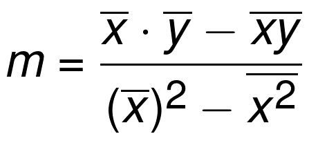
If you recall, the calculation for the best-fit/regression/'y-hat' line's slope, m:
Alright, we'll break it down into parts. First, let's grab a couple imports:
from statistics import mean
import numpy as np
We're importing mean from statistics so we can easily get the mean of a list or array. Next, we're grabbing numpy as np so that we can create NumPy arrays. We can do a lot with lists, but we need to be able to do some simple matrix operations, which aren't available with simple lists, so we'll be using NumPy. We wont be getting too complex at this stage with NumPy, but later on NumPy is going to be your best friend. Next, let's define some starting datapoints:
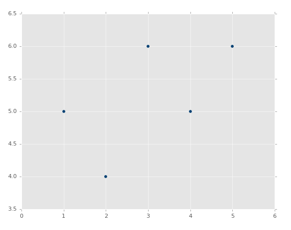
xs = [1,2,3,4,5]
ys = [5,4,6,5,6]
So these are the datapoints we're going to use, xs and ys. You can already be framing this right now as xs are the features and ys are the labels, or maybe these are both features and we're establishing a relationship. As mentioned earlier, we actually want these to be NumPy arrays so we can perform matrix operations, so let's modify those two lines:
xs = np.array([1,2,3,4,5], dtype=np.float64)
ys = np.array([5,4,6,5,6], dtype=np.float64)
Now these are numpy arrays. We're also being explicit with the datatype here. Without getting in to deep here, datatypes have certain attributes, and those attributes boil down to how the data itself is stored into memory and can be manipulated. This wont matter as much right now as it will down the line when and if we're doing massive operations and hoping to do them on our GPUs rather than CPUs.
If graphed, our data should look like:
Okay now we're ready to build a function to calculate m, which is our regression line's slope:
def best_fit_slope(xs,ys):
    return m

m = best_fit_slope(xs,ys)
Done!
Just kidding, so there's our skeleton, now we'll fill it in.
Our first order of business is to do the mean of the x points, multiplied by the mean of our y points. Continuing to fill out our skeleton:
def best_fit_slope(xs,ys):
    m = (mean(xs) * mean(ys))
    return m
Easy enough so far. You can use the mean function on lists, tuples, or arrays. Notice my use of parenthesis here. Python honors the order of operations with mathematics. So, if you're wanting to ensure order, make sure you're explicit. Remember your PEMDAS!
Next, we need to subtract the mean of x*y, which is going to be our matrix operation: mean(xs*ys). In full now:
def best_fit_slope(xs,ys):
    m = ( (mean(xs)*mean(ys)) - mean(xs*ys) )
    return m
We're done with the top part of our equation, now we're going to work on the denominator, starting with the squared mean of x: (mean(xs)*mean(xs)). While Python does support something like ^2, it's not going to work on our NumPy array float64 datatype. Adding this in:
def best_fit_slope(xs,ys):
    m = ( ((mean(xs)*mean(ys)) - mean(xs*ys)) /
           (mean(xs)**2))
    return m
While it is not necessary by the order of operations to encase the entire calculation in parenthesis, I am doing it here so I can add a new line after our division, making things a bit easier to read and follow. Without it, we'd get a syntax error at the new line. We're almost complete here, now we just need to subtract the mean of the squared x values: mean(xs*xs). Again, we can't get away with a simple carrot 2, but we can multiple the array by itself and get the same outcome we desire. All together now:
def best_fit_slope(xs,ys):
    m = (((mean(xs)*mean(ys)) - mean(xs*ys)) /
         ((mean(xs)**2) - mean(xs*xs)))
    return m
Great, our full script is now:
from statistics import mean
import numpy as np

xs = np.array([1,2,3,4,5], dtype=np.float64)
ys = np.array([5,4,6,5,6], dtype=np.float64)

def best_fit_slope(xs,ys):
    m = (((mean(xs)*mean(ys)) - mean(xs*ys)) /
         ((mean(xs)**2) - mean(xs**2)))
    return m

m = best_fit_slope(xs,ys)
print(m)
Output: 0.3
What's next? We need to calculate the y intercept: b. We will be tackling that in the next tutorial along with completing the best-fit line calculation overall. It's an easier calculation than the slope was, try to write your own function to do it. If you get it, don't skip the next tutorial, as we'll be doing more than simply calculating b.
-
Practical Machine Learning Tutorial with Python Introduction
-
Regression - Intro and Data
-
Regression - Features and Labels
-
Regression - Training and Testing
-
Regression - Forecasting and Predicting
-
Pickling and Scaling
-
Regression - Theory and how it works
-
Regression - How to program the Best Fit Slope
-
Regression - How to program the Best Fit Line
-
Regression - R Squared and Coefficient of Determination Theory
-
Regression - How to Program R Squared
-
Creating Sample Data for Testing
-
Classification Intro with K Nearest Neighbors
-
Applying K Nearest Neighbors to Data
-
Euclidean Distance theory
-
Creating a K Nearest Neighbors Classifer from scratch
-
Creating a K Nearest Neighbors Classifer from scratch part 2
-
Testing our K Nearest Neighbors classifier
-
Final thoughts on K Nearest Neighbors
-
Support Vector Machine introduction
-
Vector Basics
-
Support Vector Assertions
-
Support Vector Machine Fundamentals
-
Constraint Optimization with Support Vector Machine
-
Beginning SVM from Scratch in Python
-
Support Vector Machine Optimization in Python
-
Support Vector Machine Optimization in Python part 2
-
Visualization and Predicting with our Custom SVM
-
Kernels Introduction
-
Why Kernels
-
Soft Margin Support Vector Machine
-
Kernels, Soft Margin SVM, and Quadratic Programming with Python and CVXOPT
-
Support Vector Machine Parameters
-
Machine Learning - Clustering Introduction
-
Handling Non-Numerical Data for Machine Learning
-
K-Means with Titanic Dataset
-
K-Means from Scratch in Python
-
Finishing K-Means from Scratch in Python
-
Hierarchical Clustering with Mean Shift Introduction
-
Mean Shift applied to Titanic Dataset
-
Mean Shift algorithm from scratch in Python
-
Dynamically Weighted Bandwidth for Mean Shift
-
Introduction to Neural Networks
-
Installing TensorFlow for Deep Learning - OPTIONAL
-
Introduction to Deep Learning with TensorFlow
-
Deep Learning with TensorFlow - Creating the Neural Network Model
-
Deep Learning with TensorFlow - How the Network will run
-
Deep Learning with our own Data
-
Simple Preprocessing Language Data for Deep Learning
-
Training and Testing on our Data for Deep Learning
-
10K samples compared to 1.6 million samples with Deep Learning
-
How to use CUDA and the GPU Version of Tensorflow for Deep Learning
-
Recurrent Neural Network (RNN) basics and the Long Short Term Memory (LSTM) cell
-
RNN w/ LSTM cell example in TensorFlow and Python
-
Convolutional Neural Network (CNN) basics
-
Convolutional Neural Network CNN with TensorFlow tutorial
-
TFLearn - High Level Abstraction Layer for TensorFlow Tutorial
-
Using a 3D Convolutional Neural Network on medical imaging data (CT Scans) for Kaggle
-
Classifying Cats vs Dogs with a Convolutional Neural Network on Kaggle
-
Using a neural network to solve OpenAI's CartPole balancing environment
