Regression - Forecasting and Predicting

Welcome to part 5 of the Machine Learning with Python tutorial series, currently covering regression. Leading up to this point, we have collected data, modified it a bit, trained a classifier and even tested that classifier. In this part, we're going to use our classifier to actually do some forecasting for us! The code up to this point that we'll use:

import Quandl, math
import numpy as np
import pandas as pd
from sklearn import preprocessing, cross_validation, svm
from sklearn.linear_model import LinearRegression

df = Quandl.get("WIKI/GOOGL")
df = df[['Adj. Open',  'Adj. High',  'Adj. Low',  'Adj. Close', 'Adj. Volume']]
df['HL_PCT'] = (df['Adj. High'] - df['Adj. Low']) / df['Adj. Close'] * 100.0
df['PCT_change'] = (df['Adj. Close'] - df['Adj. Open']) / df['Adj. Open'] * 100.0

df = df[['Adj. Close', 'HL_PCT', 'PCT_change', 'Adj. Volume']]
forecast_col = 'Adj. Close'
df.fillna(value=-99999, inplace=True)
forecast_out = int(math.ceil(0.01 * len(df)))
df['label'] = df[forecast_col].shift(-forecast_out)

X = np.array(df.drop(['label'], 1))
X = preprocessing.scale(X)
X = X[:-forecast_out]
df.dropna(inplace=True)
y = np.array(df['label'])
X_train, X_test, y_train, y_test = cross_validation.train_test_split(X, y, test_size=0.2)

clf = LinearRegression(n_jobs=-1)
clf.fit(X_train, y_train)
confidence = clf.score(X_test, y_test)
print(confidence)

I will stress that creating a linear model with say >95% accuracy is not that great. I certainly wouldn't trade stocks on it. There are still many issues to consider, especially with different companies that have different price trajectories over time. Google really is very linear: Up and to the right. Many companies aren't, so keep this in mind. Now, to forecast out, we need some data. We decided that we're forecasting out 1% of the data, thus we will want to, or at least *can* generate forecasts for each of the final 1% of the dataset. So when can we do this? When would we identify that data? We could call it now, but consider the data we're trying to forecast is not scaled like the training data was. Okay, so then what? Do we just do preprocessing.scale() against the last 1%? The scale method scales based on all of the known data that is fed into it. Ideally, you would scale both the training, testing, AND forecast/predicting data all together. Is this always possible or reasonable? No. If you can do it, you should, however. In our case, right now, we can do it. Our data is small enough and the processing time is low enough, so we'll preprocess and scale the data all at once.

In many cases, you wont be able to do this. Imagine if you were using gigabytes of data to train a classifier. It may take days to train your classifier, you wouldn't want to be doing this every...single...time you wanted to make a prediction. Thus, you may need to either NOT scale anything, or you may scale the data separately. As usual, you will want to test both options and see which is best in your specific case.

With that in mind, let's handle all of the rows from the definition of X onward:

X = np.array(df.drop(['label'], 1))
X = preprocessing.scale(X)
X_lately = X[-forecast_out:]
X = X[:-forecast_out]

df.dropna(inplace=True)

y = np.array(df['label'])

X_train, X_test, y_train, y_test = cross_validation.train_test_split(X, y, test_size=0.2)
clf = LinearRegression(n_jobs=-1)
clf.fit(X_train, y_train)
confidence = clf.score(X_test, y_test)
print(confidence)

Note that first we take all data, preprocess it, and then we split it up. Our X_lately variable contains the most recent features, which we're going to predict against. As you should see so far, defining a classifier, training, and testing was all extremely simple. Predicting is also super easy:

forecast_set = clf.predict(X_lately)

The forecast_set is an array of forecasts, showing that not only could you just seek out a single prediction, but you can seek out many at once. To see what we have thus far:

print(forecast_set, confidence, forecast_out)

[ 745.67829395  737.55633261  736.32921413  717.03929303  718.59047951
  731.26376715  737.84381394  751.28161162  756.31775293  756.76751056
  763.20185946  764.52651181  760.91320031  768.0072636   766.67038016
  763.83749414  761.36173409  760.08514166  770.61581391  774.13939706
  768.78733341  775.04458624  771.10782342  765.13955723  773.93369548
  766.05507556  765.4984563   763.59630529  770.0057166   777.60915879] 0.956987938167 30

So these are our forecasts out. Now what? Well, you are basically done, but we can work on visualizing this information. So stock prices are daily, for 5 days, and then there are no prices on the weekends. I recognize this fact, but we're going to keep things simple, and plot each forecast as if it is simply 1 day out. If you want to try to work in the weekend gaps (don't forget holidays) go for it, but we'll keep it simple. To start, we'll add a couple new imports:

import datetime
import matplotlib.pyplot as plt
from matplotlib import style

We import datetime to work with datetime objects, matplotlib's pyplot package for graphing, and style to make our graphs look decent. Let's set a style:

style.use('ggplot')

Next, we're going to add a new column to our dataframe, the forecast column:

df['Forecast'] = np.nan

We set the value as a NaN first, but we'll populate some shortly. We said we're going to just start the forecasts as tomorrow (recall that we predict 10% out into the future, and we saved that last 10% of our data to do this, thus, we can begin immediately predicting since -10% has data that we can predict 10% out and be the next prediction). We need to first grab the last day in the dataframe, and begin assigning each new forecast to a new day. We will start that like so:

last_date = df.iloc[-1].name
last_unix = last_date.timestamp()
one_day = 86400
next_unix = last_unix + one_day

Now we have the next day we wish to use, and one_day is 86,400 seconds. Now we add the forecast to the existing dataframe:

for i in forecast_set:
    next_date = datetime.datetime.fromtimestamp(next_unix)
    next_unix += 86400
    df.loc[next_date] = [np.nan for _ in range(len(df.columns)-1)]+[i]

So here all we're doing is iterating through the forecast set, taking each forecast and day, and then setting those values in the dataframe (making the future "features" NaNs). The last line's code just simply takes all of the first columns, setting them to NaNs, and then the final column is whatever i is (the forecast in this case). I have chosen to do this one-liner for loop like this so that, if we decide to change up the dataframe and features, the code can still work. All that is left? Graph it!

df['Adj. Close'].plot()
df['Forecast'].plot()
plt.legend(loc=4)
plt.xlabel('Date')
plt.ylabel('Price')
plt.show()

Full code up to this point:

import Quandl, math
import numpy as np
import pandas as pd
from sklearn import preprocessing, cross_validation, svm
from sklearn.linear_model import LinearRegression
import matplotlib.pyplot as plt
from matplotlib import style
import datetime

style.use('ggplot')

df = Quandl.get("WIKI/GOOGL")
df = df[['Adj. Open',  'Adj. High',  'Adj. Low',  'Adj. Close', 'Adj. Volume']]
df['HL_PCT'] = (df['Adj. High'] - df['Adj. Low']) / df['Adj. Close'] * 100.0
df['PCT_change'] = (df['Adj. Close'] - df['Adj. Open']) / df['Adj. Open'] * 100.0

df = df[['Adj. Close', 'HL_PCT', 'PCT_change', 'Adj. Volume']]
forecast_col = 'Adj. Close'
df.fillna(value=-99999, inplace=True)
forecast_out = int(math.ceil(0.01 * len(df)))
df['label'] = df[forecast_col].shift(-forecast_out)

X = np.array(df.drop(['label'], 1))
X = preprocessing.scale(X)
X_lately = X[-forecast_out:]
X = X[:-forecast_out]

df.dropna(inplace=True)

y = np.array(df['label'])

X_train, X_test, y_train, y_test = cross_validation.train_test_split(X, y, test_size=0.2)
clf = LinearRegression(n_jobs=-1)
clf.fit(X_train, y_train)
confidence = clf.score(X_test, y_test)

forecast_set = clf.predict(X_lately)
df['Forecast'] = np.nan

last_date = df.iloc[-1].name
last_unix = last_date.timestamp()
one_day = 86400
next_unix = last_unix + one_day

for i in forecast_set:
    next_date = datetime.datetime.fromtimestamp(next_unix)
    next_unix += 86400
    df.loc[next_date] = [np.nan for _ in range(len(df.columns)-1)]+[i]

df['Adj. Close'].plot()
df['Forecast'].plot()
plt.legend(loc=4)
plt.xlabel('Date')
plt.ylabel('Price')
plt.show()

The result (I zoomed in a bit):

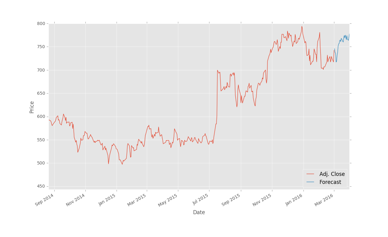
There you have it, you now have a somewhat decent method for forecasting stock prices into the future! In the next tutorial, we're going to wrap up regression with some information on saving classifiers as well as using millions of dollars worth of computational power for a few dollars.

The next tutorial: Pickling and Scaling