Creating Sample Data for Testing
Welcome to the 12th part of our Machine Learning with Python tutorial series. We've been learning about regression, and even coded our own very simple linear regression algorithm. Along with that, we've also built a coefficient of determination algorithm to check for the accuracy and reliability of our best-fit line. We've discussed and shown how a best-fit line may not be a great fit, but also explained why our example was correct directionally, even if it was not exact. Now, however, we are at the point where we're using two top-level algorithms, which are subsequently comprised of a handful of smaller algorithms. As we continue building this hierarchy of algorithms, we might wind up finding ourselves in trouble if just one of them have a tiny error, so we want to test our assumptions.
In the world of programming, the systematic testing of programs is generally called "unit testing." This is where, as a large program is built, each tiny sub-system is constantly checked. As updates and modifcations are made to a large program it can be very easy to accidentally change something that will conflict with a previous system. With machine learning, this can also be a problem, but, our main concern at this point is merely to test our assumptions. Eventually, you would be wise to create unit testing for your entire machine learning system, but, for now, we'll just keep it as simple as possible.
Our assumption is that we created a best fit line, which we then tested with a coefficient of determination method. We know (mathematically) that the r squared value will be lower when the best-fit line is worse, and higher (closer to 1), when the best fit line is better. Our assumption is that we've built a system that works this way. Our system has many parts, and even a simple order of operations error would throw everything out of the window. How could we test our algorithm's behaviors, so that we're confident everything is working as intended?
The idea here is to create a sample dataset that is defined by us. If we have a positively correlated dataset, where the correlation is quite strong and tight, then r squared should be higher, than if the correlation is weaker and points are not as tightly conformed. The easier it would be for us to personally just eye-ball and estimate the line, the better the machine should perform. Let's build a system that will generate example data that we can dictate these such parameters:
To start, we'll build a skeleton function that mimics what the end-goal is:
import random
def create_dataset(hm,variance,step=2,correlation=False):

    return np.array(xs, dtype=np.float64),np.array(ys,dtype=np.float64)
We've got the beginnings of a function that takes the following parameters:
hm - The value will be "how much." This is how many datapoints that we want in the set. We could choose to have 10, or 10 million, for example.
variance - This will dictate how much each point can vary from the previous point. The more variance, the less-tight the data will be.
step - This will be how far to step on average per point, defaulting to 2.
correlation - This will be either False, pos, or neg to indicate that we want no correlation, positive correlation, or negative correlation.
Note that we also imported random, this will help us generate seemingly random datasets.
Now we'll begin filling in the function:
def create_dataset(hm,variance,step=2,correlation=False):
    val = 1
    ys = []
    for i in range(hm):
        y = val + random.randrange(-variance,variance)
        ys.append(y)
Simple enough, we just begin iterating through the range that we chose with the hm (how much) variable, appending the current value plus a random range of the negative variance to positive variance. This gives us data, but currently no correlation if we wanted it. Let's add that:
def create_dataset(hm,variance,step=2,correlation=False):
    val = 1
    ys = []
    for i in range(hm):
        y = val + random.randrange(-variance,variance)
        ys.append(y)
        if correlation and correlation == 'pos':
            val+=step
        elif correlation and correlation == 'neg':
            val-=step
Great, now we've got a good definition for y values. Next, let's create the xs, which are much easier, then return the whole thing:
def create_dataset(hm,variance,step=2,correlation=False):
    val = 1
    ys = []
    for i in range(hm):
        y = val + random.randrange(-variance,variance)
        ys.append(y)
        if correlation and correlation == 'pos':
            val+=step
        elif correlation and correlation == 'neg':
            val-=step

    xs = [i for i in range(len(ys))]

    return np.array(xs, dtype=np.float64),np.array(ys,dtype=np.float64)
We're all set now. To create a sample dataset, all we need to do is something like:
xs, ys = create_dataset(40,40,2,correlation='pos')
Let's put it all together with the code from the previous linear regression tutorials:
from statistics import mean
import numpy as np
import random
import matplotlib.pyplot as plt
from matplotlib import style
style.use('ggplot')


def create_dataset(hm,variance,step=2,correlation=False):
    val = 1
    ys = []
    for i in range(hm):
        y = val + random.randrange(-variance,variance)
        ys.append(y)
        if correlation and correlation == 'pos':
            val+=step
        elif correlation and correlation == 'neg':
            val-=step

    xs = [i for i in range(len(ys))]

    return np.array(xs, dtype=np.float64),np.array(ys,dtype=np.float64)

def best_fit_slope_and_intercept(xs,ys):
    m = (((mean(xs)*mean(ys)) - mean(xs*ys)) /
         ((mean(xs)*mean(xs)) - mean(xs*xs)))

    b = mean(ys) - m*mean(xs)

    return m, b


def coefficient_of_determination(ys_orig,ys_line):
    y_mean_line = [mean(ys_orig) for y in ys_orig]

    squared_error_regr = sum((ys_line - ys_orig) * (ys_line - ys_orig))
    squared_error_y_mean = sum((y_mean_line - ys_orig) * (y_mean_line - ys_orig))

    print(squared_error_regr)
    print(squared_error_y_mean)

    r_squared = 1 - (squared_error_regr/squared_error_y_mean)

    return r_squared


xs, ys = create_dataset(40,40,2,correlation='pos')
m, b = best_fit_slope_and_intercept(xs,ys)
regression_line = [(m*x)+b for x in xs]
r_squared = coefficient_of_determination(ys,regression_line)
print(r_squared)

plt.scatter(xs,ys,color='#003F72', label = 'data')
plt.plot(xs, regression_line, label = 'regression line')
plt.legend(loc=4)
plt.show()
Running that exact code, you should get something similar to:
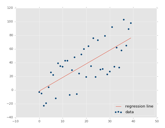
The coefficient of determination: 0.516508576011 (note that your's will not be identical, since we're using the random range).
Great, so our assumption is that our r-squared/coefficient of determination should improve if we made the dataset a more tightly correlated dataset. How would we do that? Simple: lower variance!
Using xs, ys = create_dataset(40,10,2,correlation='pos'):
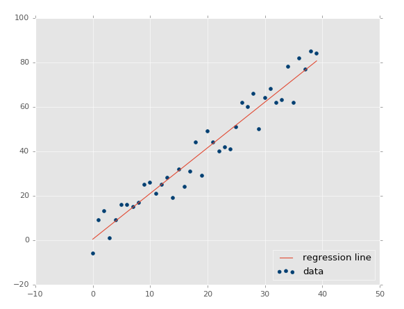
Now our r-squared value: 0.939865240568, much better, as expected. Let's test a negative correlation next:xs, ys = create_dataset(40,10,2,correlation='neg')
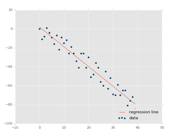
The r squared value: 0.930242442156, which is good that it is very similar to the previous one, since they had the same parameters, just opposite directions.
At this point, our assumptions are panning out and passing the test: Less variance should result in higher r-squared/coefficient of determination, higher variance = lower r squared. What about no correlation? This should be even lower, and actually quite close to zero, unless we get a crazy random permutation that actually has correlation anyway. Let's test it: xs, ys = create_dataset(40,10,2,correlation=False).
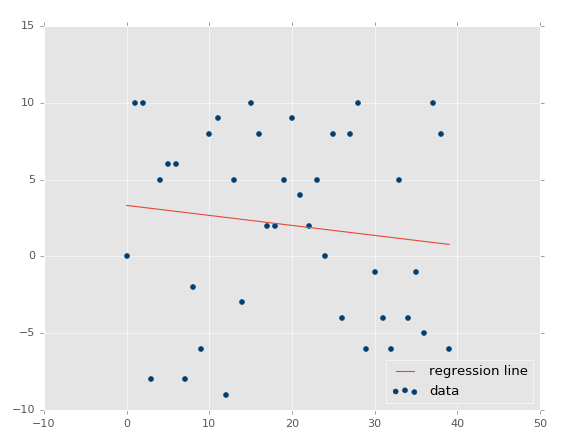
Coefficient of determination: 0.0152650900427.
By now, I think we should feel confident that things are working how we intended!
Now that you have an appreciation for simple linear regression, let's move on to classification in the next tutorial.
There exists 2 quiz/question(s) for this tutorial. for access to these, video downloads, and no ads.
-
Practical Machine Learning Tutorial with Python Introduction
-
Regression - Intro and Data
-
Regression - Features and Labels
-
Regression - Training and Testing
-
Regression - Forecasting and Predicting
-
Pickling and Scaling
-
Regression - Theory and how it works
-
Regression - How to program the Best Fit Slope
-
Regression - How to program the Best Fit Line
-
Regression - R Squared and Coefficient of Determination Theory
-
Regression - How to Program R Squared
-
Creating Sample Data for Testing
-
Classification Intro with K Nearest Neighbors
-
Applying K Nearest Neighbors to Data
-
Euclidean Distance theory
-
Creating a K Nearest Neighbors Classifer from scratch
-
Creating a K Nearest Neighbors Classifer from scratch part 2
-
Testing our K Nearest Neighbors classifier
-
Final thoughts on K Nearest Neighbors
-
Support Vector Machine introduction
-
Vector Basics
-
Support Vector Assertions
-
Support Vector Machine Fundamentals
-
Constraint Optimization with Support Vector Machine
-
Beginning SVM from Scratch in Python
-
Support Vector Machine Optimization in Python
-
Support Vector Machine Optimization in Python part 2
-
Visualization and Predicting with our Custom SVM
-
Kernels Introduction
-
Why Kernels
-
Soft Margin Support Vector Machine
-
Kernels, Soft Margin SVM, and Quadratic Programming with Python and CVXOPT
-
Support Vector Machine Parameters
-
Machine Learning - Clustering Introduction
-
Handling Non-Numerical Data for Machine Learning
-
K-Means with Titanic Dataset
-
K-Means from Scratch in Python
-
Finishing K-Means from Scratch in Python
-
Hierarchical Clustering with Mean Shift Introduction
-
Mean Shift applied to Titanic Dataset
-
Mean Shift algorithm from scratch in Python
-
Dynamically Weighted Bandwidth for Mean Shift
-
Introduction to Neural Networks
-
Installing TensorFlow for Deep Learning - OPTIONAL
-
Introduction to Deep Learning with TensorFlow
-
Deep Learning with TensorFlow - Creating the Neural Network Model
-
Deep Learning with TensorFlow - How the Network will run
-
Deep Learning with our own Data
-
Simple Preprocessing Language Data for Deep Learning
-
Training and Testing on our Data for Deep Learning
-
10K samples compared to 1.6 million samples with Deep Learning
-
How to use CUDA and the GPU Version of Tensorflow for Deep Learning
-
Recurrent Neural Network (RNN) basics and the Long Short Term Memory (LSTM) cell
-
RNN w/ LSTM cell example in TensorFlow and Python
-
Convolutional Neural Network (CNN) basics
-
Convolutional Neural Network CNN with TensorFlow tutorial
-
TFLearn - High Level Abstraction Layer for TensorFlow Tutorial
-
Using a 3D Convolutional Neural Network on medical imaging data (CT Scans) for Kaggle
-
Classifying Cats vs Dogs with a Convolutional Neural Network on Kaggle
-
Using a neural network to solve OpenAI's CartPole balancing environment
