Support Vector Machine Fundamentals

Welcome to the 23rd part of our machine learning tutorial series and the next part in our Support Vector Machine section. In this tutorial, we're going to formalize the equation for the optimization of the Support Vector Machine.

We left with the calculation of our support vectors as being: Yi(Xi.w+b)-1 = 0:

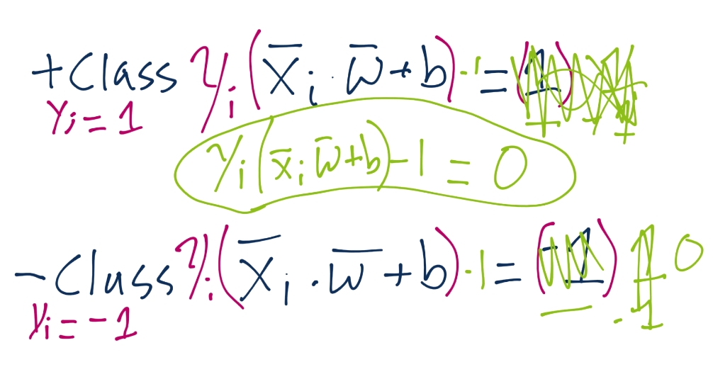
Now we're going to begin talking about how we go about the formal optimization problem of the Support Vector Machine. Specifically, how we acquire the best values for vector w and b. We'll also be covering some of the other fundamentals of the Support Vector Machine.

To start, recall the definition of a hyperplane is w.x+b. Thus, we have asserted that the definitions for the support vectors in that equation will be 1 for a positive class and -1 for a negative class:

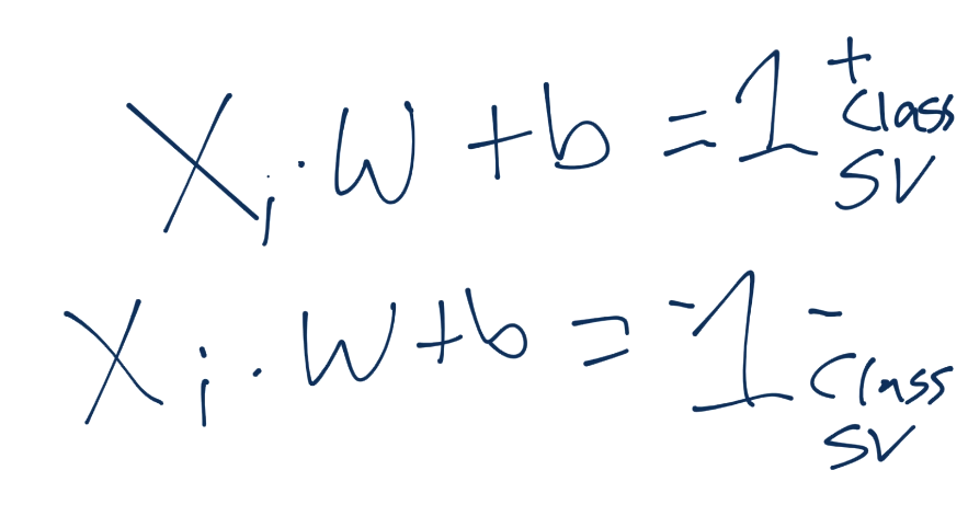
We can also surmise that, once we find a w and b to satisfy the constraint problem (the vector w with the smallest magnitude with the largest b), our decision function for classification of unknown points would just simply ask for the value of x.w+b. What if that value is 0.98? What might that look like on the graph?

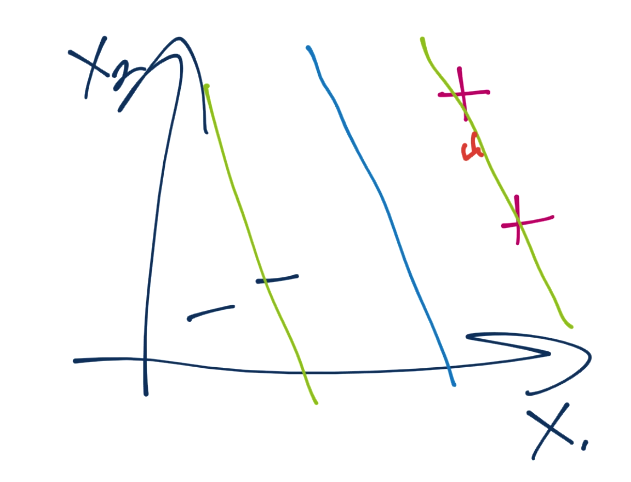
So we're not quite to the positive support vector's hyperplane, but close. Are we beyond the decision boundary? Yes, of course, which is just where x.w+b=0. Thus, the actual decision function for an unknown featureset is simply sign(x.w+b). That's it! If it's a positive, then + class. Negative? - Class. Now in order to get that function, we need w and b as we've already figured out. We have the constraint function, which is Yi(Xi.W+b) >= 1, which requires us to satisfy per featureset. How come we're requiring known features to be greater than or equal to one? Without doing the multiplication by Yi, this is basically requiring all of our known featuresets to, if passed through x.w+b to be greater than 1 or less than -1, despite us having just shown that a value of, say, 0.98, would be a positive class. The reason is, new/unkown data to be classified can be between the support vector hyperplanes and the decision boundary, but the training/known data cannot.

Thus, our goal is to minimize ||w||, maximize b, with the constraint such that Yi(Xi.W+b)>=1:

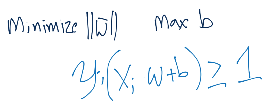
It's important to not be confused that we're trying to satisfy the constraint with the *vector* w, but minimize not the vector w, but the *magnitude* of vector w.

There are many ways to perform constraint optimization. The first method I am going to run through is the traditional depiction of the Support Vector Machine. To begin, consider we fundamentally are trying to maximize the width between separating hyperplanes:

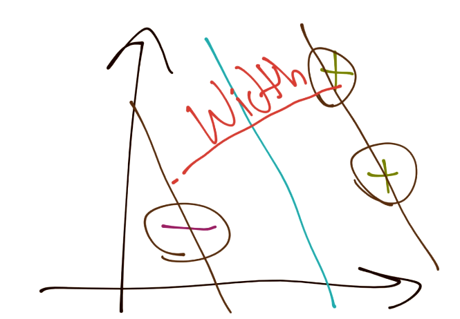
Next, the width between the vectors can be denoted as:

Notice we've got X+ and X- in there, those are the two hyperplanes we're referencing and trying to maximize the distance between. Luckily for us, there's no b here, that's nice. What about the X+ and X-, what are those? Do we know? Yeah we do! Recall:

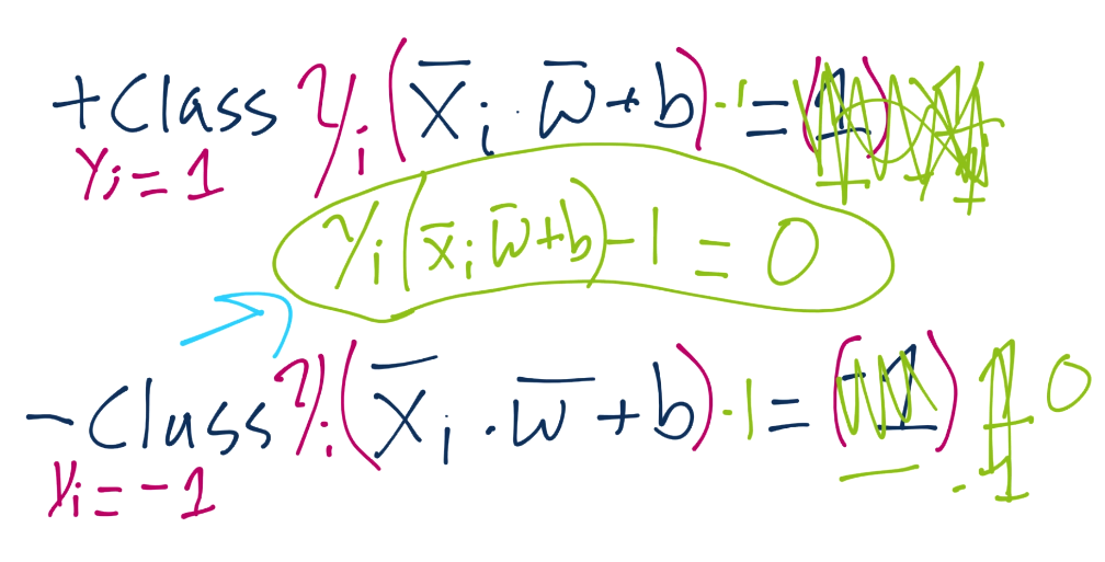
...and there's the b. One day, we're going to solve for that. Anyway, we'll plug in the equations, do the algebra, and we get that X+ and X- are essentially 1-b and 1+b.

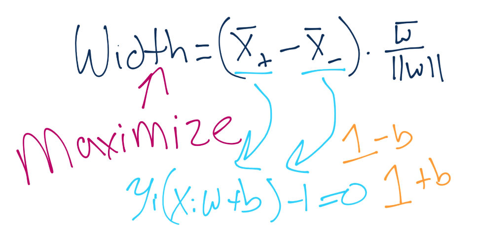
Remember your order of operations? Isn't this convenient, we get to tell b to go away again, and now our equation for width gets simplified:

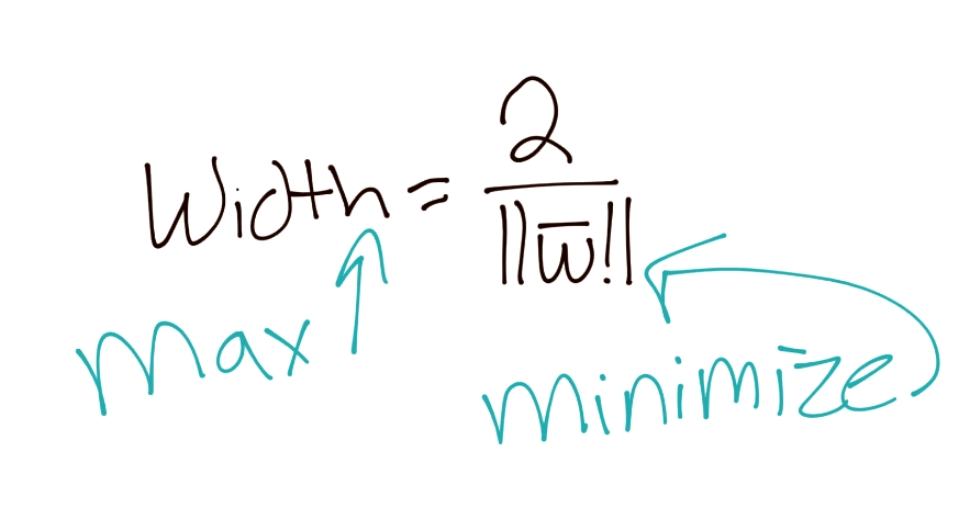
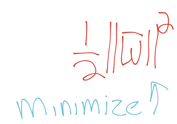
Then to better suit our needs in the future, we're going to assert that, if we want to maximize 2/||w||, then we also obviously want to minimize ||w||, which we've already stated. Since we want to minimize ||w||, we also would want to minimize, say, 1/2||w||^2:

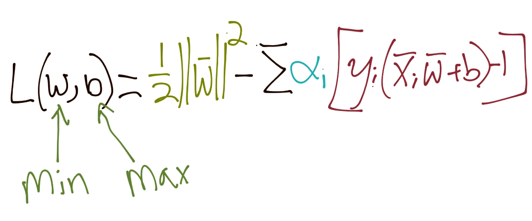
We're doing that, along with our constraint that: Yi(Xi.W+b)-1 = 0. Thus, the sum of ALL of the featuresets should meet that constraint of 0 still. So we introduce the lagrangian constraint optimization problem:

Doing the derivatives here

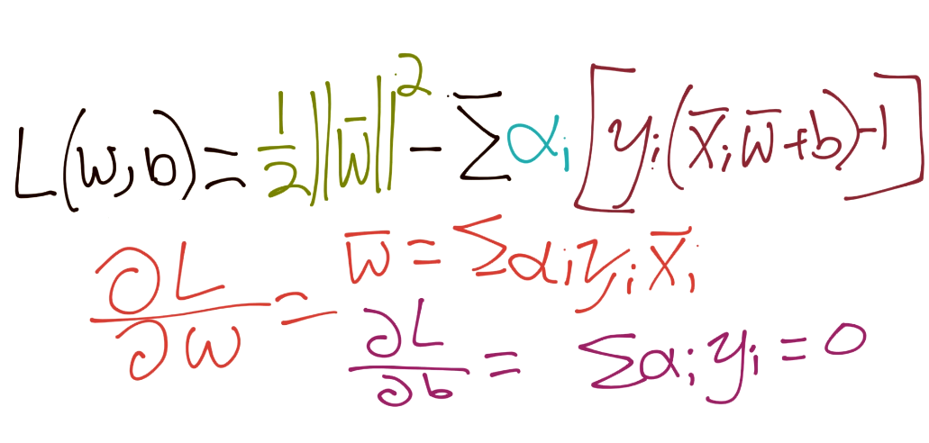
Putting back together:

Thus, if you're not already unhappy with the way things have turned, now you are. We've got alpha squared, which means we've got ourselves a quadratic programming problem to solve.

Well that escalated quickly.

In the next tutorial, given our interest in writing the SVM from scratch in code, we're going to see if we can simplify things a bit.

The next tutorial: Constraint Optimization with Support Vector Machine