Annotating Last Price Stock Chart with Matplotlib

In this Matplotlib tutorial, we're going to show an example of how we can track the last price of a stock, by annotating it to the right side of the axis like a lot of charting applications will do.

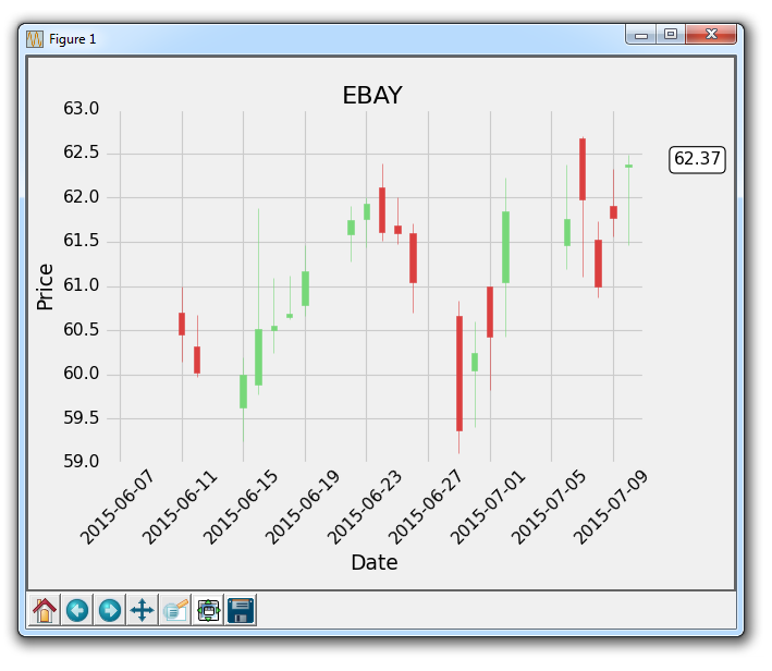
While people like to see historical prices in their live graphs, they also want to see the most recent price. What most applications do, is the annotate the last price at the y-axis height of the price, and then kind of highlight it and move it around a bit in a box of sorts as price changes. Using our recently-learned annotation tutorial, we can do this along with adding a bbox.

The crux of our code is:

    bbox_props = dict(boxstyle='round',fc='w', ec='k',lw=1)
    
    ax1.annotate(str(closep[-1]), (date[-1], closep[-1]),
                 xytext = (date[-1]+4, closep[-1]), bbox=bbox_props)

We use ax1.annotate to place the string value of the last price. We aren't using it really here, but we specify the plot that we're annotating as the last plot. Next, we use xytext to place our text to a specific location. We place it where the last price is on the Y axis, then we place it at the last x, plus a few points. We do this to move it off the graph. This is enough to place the text off the graph, but right now it's just some floating text.

We use the bbox parameter to create a box around the text. We use bbox_props to create a property dict, containing a box style, then a white (w) face color, a black (k) edge color, and a line width of one. For more box styles, see the matplotlib documentation for annotations.

Finally, this annotation being over to the right a bit requires us to make some new space with subplots_adjust:

    plt.subplots_adjust(left=0.11, bottom=0.24, right=0.87, top=0.90, wspace=0.2, hspace=0)

The full code up to this point would be:

import matplotlib.pyplot as plt
import matplotlib.dates as mdates
import matplotlib.ticker as mticker
from matplotlib.finance import candlestick_ohlc
from matplotlib import style

import numpy as np
import urllib
import datetime as dt

style.use('fivethirtyeight')
print(plt.style.available)

print(plt.__file__)


def bytespdate2num(fmt, encoding='utf-8'):
    strconverter = mdates.strpdate2num(fmt)
    def bytesconverter(b):
        s = b.decode(encoding)
        return strconverter(s)
    return bytesconverter
    

def graph_data(stock):

    fig = plt.figure()
    ax1 = plt.subplot2grid((1,1), (0,0))
    
    stock_price_url = 'http://chartapi.finance.yahoo.com/instrument/1.0/'+stock+'/chartdata;type=quote;range=1m/csv'
    source_code = urllib.request.urlopen(stock_price_url).read().decode()
    stock_data = []
    split_source = source_code.split('\n')
    for line in split_source:
        split_line = line.split(',')
        if len(split_line) == 6:
            if 'values' not in line and 'labels' not in line:
                stock_data.append(line)

    
    date, closep, highp, lowp, openp, volume = np.loadtxt(stock_data,
                                                          delimiter=',',
                                                          unpack=True,
                                                          converters={0: bytespdate2num('%Y%m%d')})

    x = 0
    y = len(date)
    ohlc = []

    while x < y:
        append_me = date[x], openp[x], highp[x], lowp[x], closep[x], volume[x]
        ohlc.append(append_me)
        x+=1


    candlestick_ohlc(ax1, ohlc, width=0.4, colorup='#77d879', colordown='#db3f3f')
  
    for label in ax1.xaxis.get_ticklabels():
        label.set_rotation(45)

    ax1.xaxis.set_major_formatter(mdates.DateFormatter('%Y-%m-%d'))
    ax1.xaxis.set_major_locator(mticker.MaxNLocator(10))
    ax1.grid(True)
    
    bbox_props = dict(boxstyle='round',fc='w', ec='k',lw=1)
    
    ax1.annotate(str(closep[-1]), (date[-1], closep[-1]),
                 xytext = (date[-1]+3, closep[-1]), bbox=bbox_props)

    
##    # Annotation example with arrow
##    ax1.annotate('Bad News!',(date[11],highp[11]),
##                 xytext=(0.8, 0.9), textcoords='axes fraction',
##                 arrowprops = dict(facecolor='grey',color='grey'))
##
##    
##    # Font dict example
##    font_dict = {'family':'serif',
##                 'color':'darkred',
##                 'size':15}
##    # Hard coded text 
##    ax1.text(date[10], closep[1],'Text Example', fontdict=font_dict)

    plt.xlabel('Date')
    plt.ylabel('Price')
    plt.title(stock)
    #plt.legend()
    plt.subplots_adjust(left=0.11, bottom=0.24, right=0.87, top=0.90, wspace=0.2, hspace=0)
    plt.show()


graph_data('EBAY')

With the result:

The next tutorial: Subplots with Matplotlib