Zipline backtest visualization - Python Programming for Finance p.26

Welcome to part 2 of the local backtesting with Zipline tutorial series. In the previous tutorial, we've installed Zipline and run a backtest, seeing that the return is a dataframe with all sorts of information for us. We're going to now see how we can interact with this to visualize our results.

Up to this point, our script has the following:

Required IPython magic for zipline:

%load_ext zipline

Then:

from zipline.api import order, record, symbol


def initialize(context):
    pass


def handle_data(context, data):
    order(symbol('AAPL'), 10)
    record(AAPL=data.current(symbol('AAPL'), 'price'))

To run, we used:

%zipline --bundle quantopian-quandl --start 2000-1-1 --end 2012-1-1 -o backtest.pickle, you also could use zipline.exe to run things. The return here is a pandas dataframe, which we also stored to backtest.pickle.

Now, we have a few options. One is to just load in the dataframe and visualize it. For example:

import pandas as pd
import matplotlib.pyplot as plt
from matplotlib import style


style.use('ggplot')

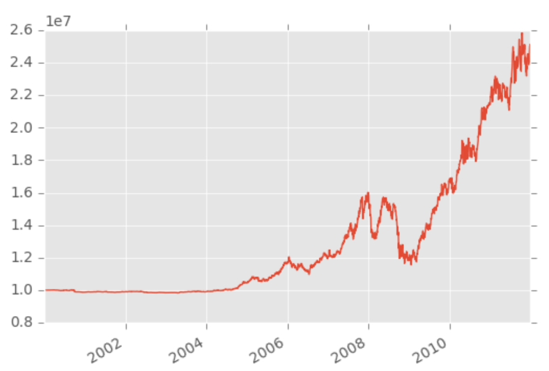
backtest_df = pd.read_pickle("backtest.pickle")
backtest_df.portfolio_value.plot()
plt.show()

That's just one quick example. We can also do:

backtest_df.columns

...seeing that we have quite a few things that are automatically tracked for us:

Index(['AAPL', 'algo_volatility', 'algorithm_period_return', 'alpha',
       'benchmark_period_return', 'benchmark_volatility', 'beta',
       'capital_used', 'ending_cash', 'ending_exposure', 'ending_value',
       'excess_return', 'gross_leverage', 'long_exposure', 'long_value',
       'longs_count', 'max_drawdown', 'max_leverage', 'net_leverage', 'orders',
       'period_close', 'period_label', 'period_open', 'pnl', 'portfolio_value',
       'positions', 'returns', 'sharpe', 'short_exposure', 'short_value',
       'shorts_count', 'sortino', 'starting_cash', 'starting_exposure',
       'starting_value', 'trading_days', 'transactions',
       'treasury_period_return'],
      dtype='object')

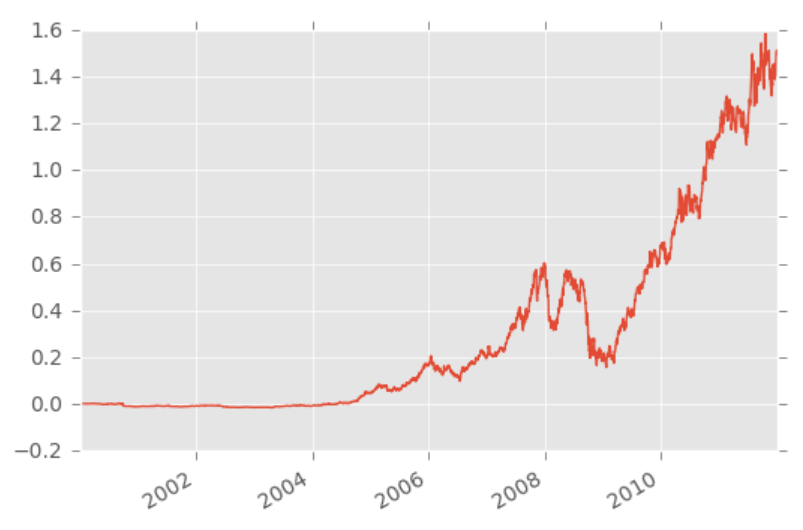
Just like in Quantopian, we can also use the record function to record more data to our output. We can also perform modifications to the dataframe, something like:

backtest_df.portfolio_value.pct_change().fillna(0).add(1).cumprod().sub(1).plot()
plt.show()

Another option you have to visualize things is automatically with an analyze function.

from zipline.api import order, record, symbol
import matplotlib.pyplot as plt
from matplotlib import style

style.use('ggplot')


def initialize(context):
    pass


def handle_data(context, data):
    order(symbol("AAPL"), 10)
    record(AAPL=data.current(symbol('EBAY'), 'price'))


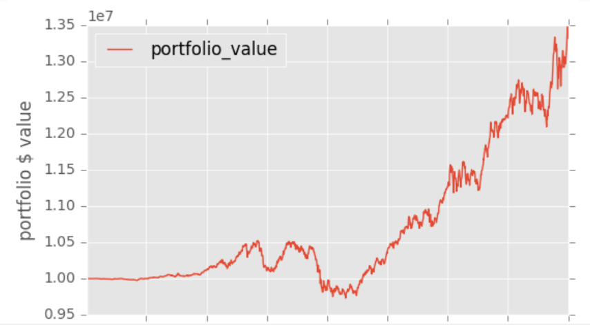
def analyze(context, perf):
    fig = plt.figure()
    ax1 = fig.add_subplot(111)
    perf.portfolio_value.plot(ax=ax1)
    ax1.set_ylabel('portfolio $ value')
    plt.legend(loc=0)
    plt.show()    

%zipline --bundle quantopian-quandl --start 2001-1-1 --end 2005-1-1 -o backtest.pickle

I have personally found that I prefer to keep the backtest and visualization separated, so I can tinker around with the results, rather than needing to re-run everything just to visualize various different things, but, once you have solidified exactly what you want to see, the analyze function could save some time.

Anyway, up to this point, we've just used some pre-bundled data, and one of the major reasons why we might want to use Zipline locally is to use our own data, so let's work on doing that in the next tutorial!

The next tutorial: Custom Data with Zipline Local - Python Programming for Finance p.27