Custom Data with Zipline Local - Python Programming for Finance p.27
Welcome to part 3 of the local backtesting with Zipline tutorial series. So far, we've shown how to run Zipline locally, but we've been using a pre-made dataset. In this tutorial, we're going to cover how you can use local data, so long as you can fit that local data into your memory. Zipline has the ability to support you using data that exhausts your available memory (such as for high-frequency trading), but this method is overly complex if you have data that *does* fit into memory like minute (as long as you don't track a huge number of assets I suppose), hourly, or especially daily data.
It took me quite a while to figure out, but, it turns out loading data to use locally for trading isn't all that bad.
I am going to have us use SPY.csv as some sample data, but I encourage you to use *any* OHLC+volume data that you have. I provide the SPY.csv file in case you want to follow along exactly, or you don't have a local dataset at the moment, but the idea is that you can use any data you like! In our case, this is also just data for a single ticker, the SPY (S&P 500 ETF), but you could also load in many other tickers/assets. Later on, I will have us using cryptocurrency data, for example.
We need data with OHLC (open, high, low, close) and volume data. We will have dataframes, per ticker, with this information. Then, we combine multiple dataframes into what is called a panel.
To begin:
import pandas as pd
from collections import OrderedDict
import pytz

full_file_path = "SPY.csv"
data = OrderedDict()
data['SPY'] = pd.read_csv(full_file_path, index_col=0, parse_dates=['date'])
data['SPY'] = data['SPY'][["open","high","low","close","volume"]]
print(data['SPY'].head())
              close
date
1993-01-29  43.9375
1993-02-01  44.2500
1993-02-02  44.3437
1993-02-03  44.8125
1993-02-04  45.0000
You can change the file path with whatever you like, this is just an example. Do note that your column names need to be the same. Lower-cased, open, high, low, close, volume, and date. For each of the data[TICKERS], you could have many more than just "SPY." In this case, I am just going to put in one ticker, but you can imagine how you might loop through a series of tickers, loading in the data one-by-one into the data variable.
Whenever you have all of your dataframes stored in this dictionary, you can then convert it to a panel, like so:
panel = pd.Panel(data)
panel.minor_axis = ["open","high","low","close","volume"]
panel.major_axis = panel.major_axis.tz_localize(pytz.utc)
print(panel)
With this panel now, we can actually pass this as our "data" to our backtest, like this:
from zipline.api import order, record, symbol, set_benchmark
import zipline
import matplotlib.pyplot as plt
from datetime import datetime


def initialize(context):
    set_benchmark(symbol("SPY"))


def handle_data(context, data):
    order(symbol("SPY"), 10)
    record(SPY=data.current(symbol('SPY'), 'price'))

perf = zipline.run_algorithm(start=datetime(2017, 1, 5, 0, 0, 0, 0, pytz.utc),
                      end=datetime(2018, 3, 1, 0, 0, 0, 0, pytz.utc),
                      initialize=initialize,
                      capital_base=100000,
                      handle_data=handle_data,
                      data=panel)
Did you hit something like
KeyError: 'the label [2017-01-07 00:00:00+00:00] is not in the [index]'
If so, it's probably because you're trying to trade something that isn't quite on the NYSE trading calendar, such as a different market. We're going to cover this in the next tutorial, how to do it propery, but, for the time being, one fix could be doing something like:
data = OrderedDict()
data['SPY'] = pd.read_csv(full_file_path, index_col=0, parse_dates=['date'])
data['SPY'] = data['SPY'][["open","high","low","close","volume"]]
data['SPY'] = data['SPY'].resample("1d").mean()
data['SPY'].fillna(method="ffill", inplace=True)
print(data['SPY'].head())
This way, you have data for every day. It shouldn't be necessary if you're following with us, but it would be otherwise. Anyway, continuing along:
import matplotlib.pyplot as plt
from matplotlib import style


style.use("ggplot")

perf.portfolio_value.pct_change().fillna(0).add(1).cumprod().sub(1).plot(label='portfolio')
perf.SPY.pct_change().fillna(0).add(1).cumprod().sub(1).plot(label='benchmark')
plt.legend(loc=2)

plt.show()
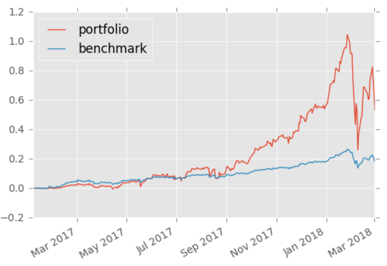
Wow, we're investment gods!
perf.max_leverage.plot()
plt.show()
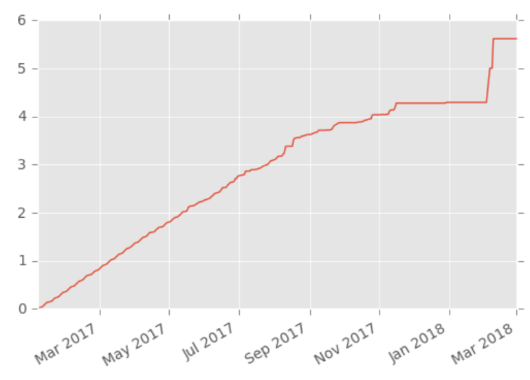
Oh right. This is of course because we keep buying 10 shares every chance we get! In case you've skipped the quantopian tutorials, you may want to go back to the first few, especially this one: placing a trade, which goes over some of the things you need to watch out for when trading. Zipline does *whatever* you ask, so you have to make sure your requests are wise and logical, just like any other program you might write..
Now, this tutorial is enough if you intend to just trade the US stock market on the NYSE trading days, but what if you have a market outside of the US? What about forex? What about cryptocurrencies? In the next tutorial, I will show you how you can go about modifying the calendars to trade any market you wish.
-
Intro and Getting Stock Price Data - Python Programming for Finance p.1
-
Handling Data and Graphing - Python Programming for Finance p.2
-
Basic stock data Manipulation - Python Programming for Finance p.3
-
More stock manipulations - Python Programming for Finance p.4
-
Automating getting the S&P 500 list - Python Programming for Finance p.5
-
Getting all company pricing data in the S&P 500 - Python Programming for Finance p.6
-
Combining all S&P 500 company prices into one DataFrame - Python Programming for Finance p.7
-
Creating massive S&P 500 company correlation table for Relationships - Python Programming for Finance p.8
-
Preprocessing data to prepare for Machine Learning with stock data - Python Programming for Finance p.9
-
Creating targets for machine learning labels - Python Programming for Finance p.10 and 11
-
Machine learning against S&P 500 company prices - Python Programming for Finance p.12
-
Testing trading strategies with Quantopian Introduction - Python Programming for Finance p.13
-
Placing a trade order with Quantopian - Python Programming for Finance p.14
-
Scheduling a function on Quantopian - Python Programming for Finance p.15
-
Quantopian Research Introduction - Python Programming for Finance p.16
-
Quantopian Pipeline - Python Programming for Finance p.17
-
Alphalens on Quantopian - Python Programming for Finance p.18
-
Back testing our Alpha Factor on Quantopian - Python Programming for Finance p.19
-
Analyzing Quantopian strategy back test results with Pyfolio - Python Programming for Finance p.20
-
Strategizing - Python Programming for Finance p.21
-
Finding more Alpha Factors - Python Programming for Finance p.22
-
Combining Alpha Factors - Python Programming for Finance p.23
-
Portfolio Optimization - Python Programming for Finance p.24
-
Zipline Local Installation for backtesting - Python Programming for Finance p.25
-
Zipline backtest visualization - Python Programming for Finance p.26
-
Custom Data with Zipline Local - Python Programming for Finance p.27
-
Custom Markets Trading Calendar with Zipline (Bitcoin/cryptocurrency example) - Python Programming for Finance p.28
