Basics for a Strategy

import datetime
import pandas as pd
import pandas.io.data
from pandas import Series, DataFrame
import matplotlib.pyplot as plt
import matplotlib as mpl
import matplotlib.ticker as mticker
import matplotlib.dates as mdates
from matplotlib import style
import numpy as np
import time

style.use('ggplot')

def outlier_fixing(stock_name,ma1=100,ma2=250,ma3=500,ma4=5000):

    df = pd.read_csv('X:/stocks_sentdex_dates_short.csv', index_col='time', parse_dates=True)
    print df.head()

    df = df[df.type == stock_name.lower()]

    std = pd.rolling_std(df['close'], 25, min_periods=1)
    print std

    df['std'] = pd.rolling_std(df['close'], 25, min_periods=1)

    df = df[df['std'] < 17]
    
    MA1 = pd.rolling_mean(df['value'], ma1)
    MA2 = pd.rolling_mean(df['value'], ma2)
    MA3 = pd.rolling_mean(df['value'], ma3)
    MA4 = pd.rolling_mean(df['value'], ma4)
    
    ax1 = plt.subplot(3, 1, 1)
    df['close'].plot(label='Price')
    
    ax2 = plt.subplot(3, 1, 2, sharex = ax1)
    MA1.plot(label=(str(ma1)+'MA'))
    MA2.plot(label=(str(ma2)+'MA'))
    MA3.plot(label=(str(ma3)+'MA'))
    MA4.plot(label=(str(ma4)+'MA'))

    ax3 = plt.subplot(3, 1, 3, sharex = ax1)
    df['std'].plot(label='Deviation')

    plt.legend()
    plt.show()
    
#outlier_fixing('btcusd',ma1=100,ma2=2500,ma3=5000,ma4=50000)

def single_stock(stock_name,ma1=100,ma2=250,ma3=500,ma4=5000):

    df = pd.read_csv('X:/stocks_sentdex_dates_full.csv', index_col='time', parse_dates=True)
    print df.head()

    df = df[df.type == stock_name.lower()]

    MA1 = pd.rolling_mean(df['value'], ma1)
    MA2 = pd.rolling_mean(df['value'], ma2)
    MA3 = pd.rolling_mean(df['value'], ma3)
    MA4 = pd.rolling_mean(df['value'], ma4)
    

    ax1 = plt.subplot(2, 1, 1)
    df['close'].plot(label='Price')
    
    ax2 = plt.subplot(2, 1, 2, sharex = ax1)
    MA1.plot(label=(str(ma1)+'MA'))
    MA2.plot(label=(str(ma2)+'MA'))
    MA3.plot(label=(str(ma3)+'MA'))
    MA4.plot(label=(str(ma4)+'MA'))

    plt.legend()
    plt.show()


def single_stock_auto_MA(stock_name):

    df = pd.read_csv('X:/stocks_sentdex_dates_full.csv',
                     index_col='time', parse_dates=True)
    print df.head()

    df = df[df.type == stock_name.lower()]
    print '----'
    count = df['type'].value_counts()
    print 'trying:' 
    count = int(count[stock_name])
    
    MA1 = pd.rolling_mean(df['value'], (count/275))
    MA2 = pd.rolling_mean(df['value'], (count/110))
    MA3 = pd.rolling_mean(df['value'], (count/55))
    # because we use a decimal here, and we're using py 2.7, this will
    # create a float as opposed to the others that will create an int
    MA4 = pd.rolling_mean(df['value'], (count/5.5))
    

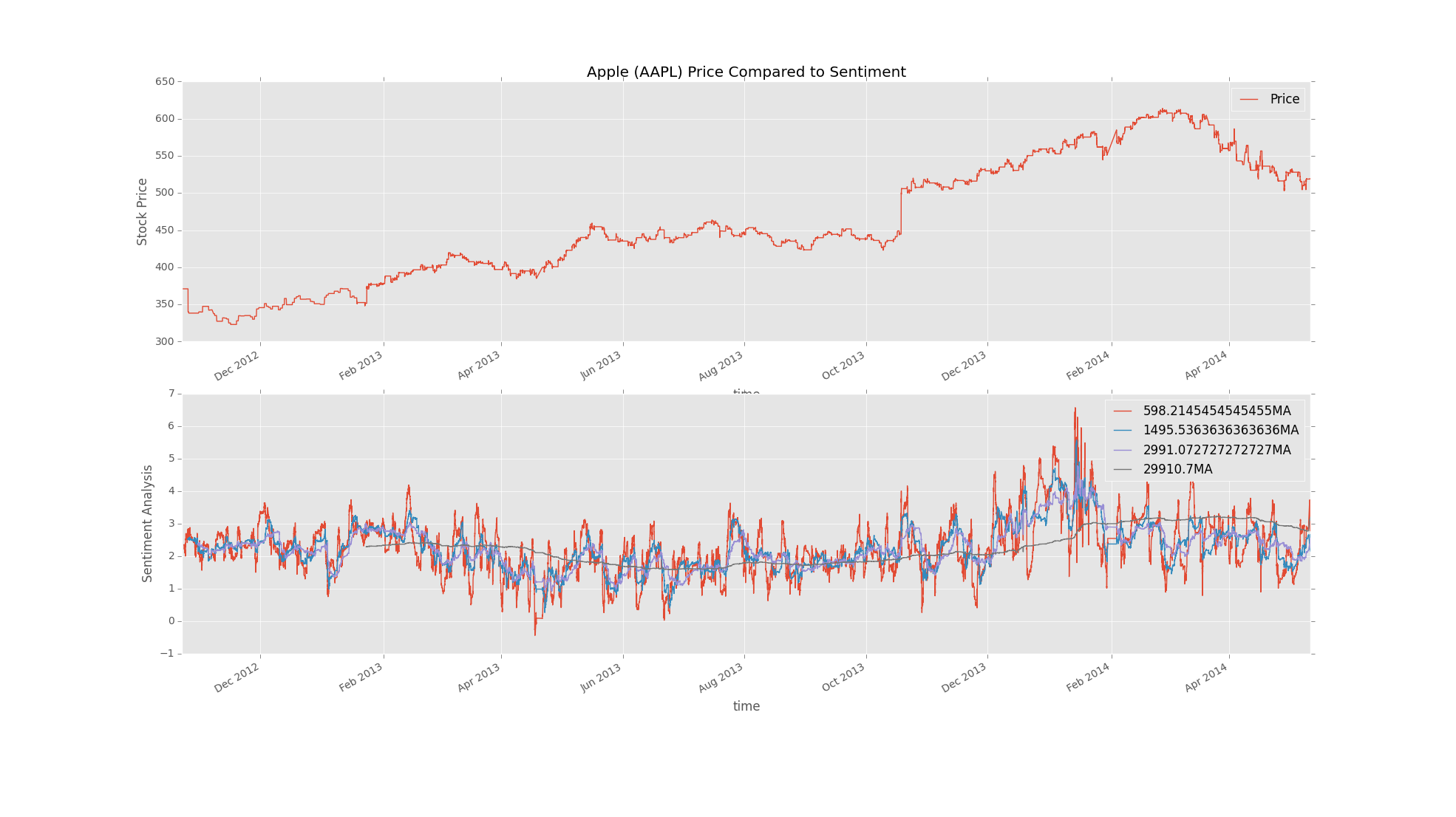
    ax1 = plt.subplot(2, 1, 1)
    df['close'].plot(label='Price')
    plt.ylabel('Stock Price')
    plt.legend()
    plt.title('Apple (AAPL) Price Compared to Sentiment')
    
    ax2 = plt.subplot(2, 1, 2, sharex = ax1)
    MA1.plot(label=(str(count/275)+'MA'))
    MA2.plot(label=(str(count/110)+'MA'))
    MA3.plot(label=(str(count/55)+'MA'))
    MA4.plot(label=(str(round((count/5.5), 1))+'MA'))
    plt.ylabel('Sentiment Analysis')

    plt.legend()
    plt.show()


#single_stock_auto_MA('c')
single_stock_auto_MA('goog')
#single_stock_auto_MA('aapl')




		

The next tutorial: Dynamic Moving Averages