Testing our Machine Learning Strategy - Python for Finance 17
Algorithmic trading with Python Tutorial
Now that we have our machine learning classifier making predictions, we're ready to see how they do! Doing this final step is fairly easy:
            if p == 1:
                order_target_percent(stock,0.11)
            elif p == -1:
                order_target_percent(stock,-0.11)
That's all there is to it. The full code is:
from sklearn.linear_model import LogisticRegression
from sklearn.svm import SVC, LinearSVC, NuSVC
from sklearn.ensemble import RandomForestClassifier
from sklearn import preprocessing
from collections import Counter
import numpy as np


def initialize(context):

    context.stocks = symbols('XLY',  # XLY Consumer Discrectionary SPDR Fund
                           'XLF',  # XLF Financial SPDR Fund
                           'XLK',  # XLK Technology SPDR Fund
                           'XLE',  # XLE Energy SPDR Fund
                           'XLV',  # XLV Health Care SPRD Fund
                           'XLI',  # XLI Industrial SPDR Fund
                           'XLP',  # XLP Consumer Staples SPDR Fund
                           'XLB',  # XLB Materials SPDR Fund
                           'XLU')  # XLU Utilities SPRD Fund

    context.historical_bars = 100
    context.feature_window = 10


def handle_data(context, data):
    prices = history(bar_count = context.historical_bars, frequency='1d', field='price')

    for stock in context.stocks:
        try:
            ma1 = data[stock].mavg(50)
            ma2 = data[stock].mavg(200)

            start_bar = context.feature_window
            price_list = prices[stock].tolist()

            X = []
            y = []

            bar = start_bar

            # feature creation
            while bar < len(price_list)-1:
                try:
                    end_price = price_list[bar+1]
                    begin_price = price_list[bar]

                    pricing_list = []
                    xx = 0
                    for _ in range(context.feature_window):
                        price = price_list[bar-(context.feature_window-xx)]
                        pricing_list.append(price)
                        xx += 1

                    features = np.around(np.diff(pricing_list) / pricing_list[:-1] * 100.0, 1)


                    #print(features)

                    if end_price > begin_price:
                        label = 1
                    else:
                        label = -1

                    bar += 1
                    X.append(features)
                    y.append(label)

                except Exception as e:
                    bar += 1
                    print(('feature creation',str(e)))


            clf = RandomForestClassifier()

            last_prices = price_list[-context.feature_window:]
            current_features = np.around(np.diff(last_prices) / last_prices[:-1] * 100.0, 1)

            X.append(current_features)
            X = preprocessing.scale(X)

            current_features = X[-1]
            X = X[:-1]

            clf.fit(X,y)
            p = clf.predict(current_features)[0]

            print(('Prediction',p))
            if p == 1:
                order_target_percent(stock,0.11)
            elif p == -1:
                order_target_percent(stock,-0.11)

        except Exception as e:
            print(str(e))


    record('ma1',ma1)
    record('ma2',ma2)
    record('Leverage',context.account.leverage)
Unfortunately, building this:
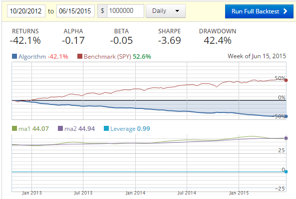
Ouch.
Now what? First, we could re-query our old friends, the moving averages, which will either confirm or deny our choices for us. Something like:
            if p == 1 and ma1 > ma2:
                order_target_percent(stock,0.11)
            elif p == -1 and ma1 < ma2:
                order_target_percent(stock,-0.11)
Giving us:
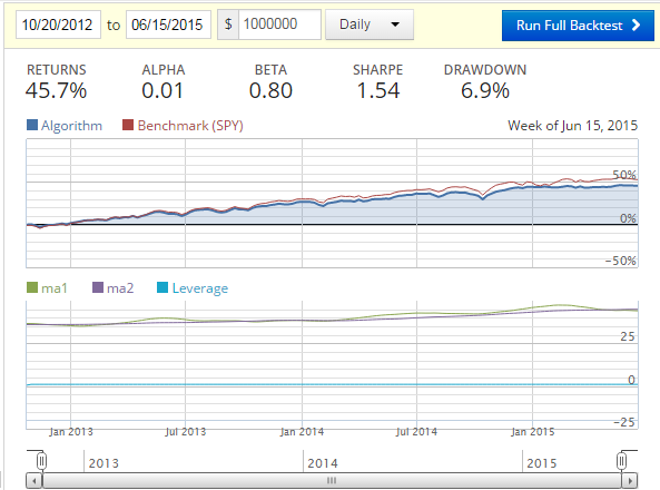
Of course, we need to ask ourselves what about just a moving average for this time period?
            if ma1 > ma2:
                order_target_percent(stock,0.11)
            elif ma1 < ma2:
                order_target_percent(stock,-0.11)
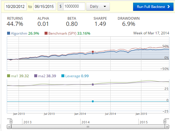
Fairly close returns, but our additional machine learning code did earn us 1% more, and gave us a 3.3% better Sharpe Ratio. Not much, but also not something to just ignore. What if we add more algorithms to the mix?
What we can do is use multiple classifiers to "vote" on the move we should make. We could end up taking the mode of the return from the classifiers, which is very much an Ensemble method, and very closely related to how the Random Forest classifier works. That said, we can use algorithms that are slightly different, so we're not being redundant. We can also require all classifiers to be in agreement, or even require a certain percentage or number of them to be in agreement. Here, we'll require all four classifiers to be in agreement.
We've already imported the other classifiers that we'd like to use, so now we just need to incorporate them into the code. Forgetting the existence of for loops for a bit:
            clf1 = RandomForestClassifier()
            clf2 = LinearSVC()
            clf3 = NuSVC()
            clf4 = LogisticRegression()

            last_prices = price_list[-context.feature_window:]
            current_features = np.around(np.diff(last_prices) / last_prices[:-1] * 100.0, 1)

            X.append(current_features)
            X = preprocessing.scale(X)

            current_features = X[-1]
            X = X[:-1]

            clf1.fit(X,y)
            clf2.fit(X,y)
            clf3.fit(X,y)
            clf4.fit(X,y)

            p1 = clf1.predict(current_features)[0]
            p2 = clf2.predict(current_features)[0]
            p3 = clf3.predict(current_features)[0]
            p4 = clf4.predict(current_features)[0]


            if Counter([p1,p2,p3,p4]).most_common(1)[0][1] >= 4:
                p = Counter([p1,p2,p3,p4]).most_common(1)[0][0]

            else:
                p = 0

            print(('Prediction',p))


            if p == 1 and ma1 > ma2:
                order_target_percent(stock,0.11)
            elif p == -1 and ma1 < ma2:
                order_target_percent(stock,-0.11)
Running this:

Now we've got a 3.28% increase in the performance percent from the previous step, and another 3.2% gain in the Sharpe Ratio from the previous step.
Overall, from a basic moving average to the multiple machine learning classifiers, we see a 5.6% improvement in the performance percent (or a 2.5% performance gain), and a 6.7% increase in the Sharpe Ratio.
These may seem like minor changes, but, not only can they make a big monetary difference, they can also tell us we're on the right track.
What if we apply leverage? Let's apply 3 to 1:
            if p == 1 and ma1 > ma2:
                order_target_percent(stock,0.33)
            elif p == -1 and ma1 < ma2:
                order_target_percent(stock,-0.33)
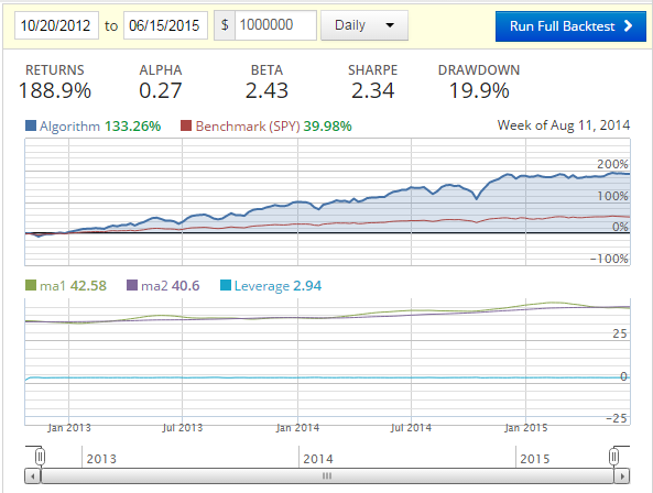
Interesting. Is leverage a magical "earn more money" kind of thing? That's what we'll be talking about in the next tutorial.
-
Programming for Finance with Python, Zipline and Quantopian
-
Programming for Finance Part 2 - Creating an automated trading strategy
-
Programming for Finance Part 3 - Back Testing Strategy
-
Accessing Fundamental company Data - Programming for Finance with Python - Part 4
-
Back-testing our strategy - Programming for Finance with Python - part 5
-
Strategy Sell Logic with Schedule Function with Quantopian - Python for Finance 6
-
Stop-Loss in our trading strategy - Python for Finance with Quantopian and Zipline 7
-
Achieving Targets - Python for Finance with Zipline and Quantopian 8
-
Quantopian Fetcher - Python for Finance with Zipline and Quantopian 9
-
Trading Logic with Sentiment Analysis Signals - Python for Finance 10
-
Shorting based on Sentiment Analysis signals - Python for Finance 11
-
Paper Trading a Strategy on Quantopian - Python for Finance 12
-
Understanding Hedgefund and other financial Objectives - Python for Finance 13
-
Building Machine Learning Framework - Python for Finance 14
-
Creating Machine Learning Classifier Feature Sets - Python for Finance 15
-
Creating our Machine Learning Classifiers - Python for Finance 16
-
Testing our Machine Learning Strategy - Python for Finance 17
-
Understanding Leverage - Python for Finance 18
-
Quantopian Pipeline Tutorial Introduction
-
Simple Quantopian Pipeline Strategy
