Portfolio Optimization - Python Programming for Finance p.24
Welcome to part 12 of the algorithmic trading with Python and Quantopian tutorials. In this tutorial, we're going to cover the portfolio construction step of the Quantopian trading strategy workflow. In the previous videos, we've covered how to find alpha factors, how to combine them, and how to analyze combined alpha factors. We've discovered that the combination of alpha factors is better than any one of the factors, and now we're ready to actually try to back test these factors in a trading situation.
First, let's just test how these factors do, using the quantiles grouping method for portfolio construction from before. To do this, we're starting with the algorithm from the part 7 strategy backtest:
from quantopian.pipeline import Pipeline
from quantopian.algorithm import attach_pipeline, pipeline_output
from quantopian.pipeline.filters.morningstar import Q1500US
from quantopian.pipeline.data.sentdex import sentiment

def initialize(context):
    """
    Called once at the start of the algorithm.
    """
    # Rebalance every day, 1 hour after market open.
    schedule_function(my_rebalance, date_rules.every_day(), time_rules.market_open(hours=1))

    # Record tracking variables at the end of each day.
    schedule_function(my_record_vars, date_rules.every_day(), time_rules.market_close())

    # Create our dynamic stock selector.
    attach_pipeline(make_pipeline(), 'my_pipeline')

    set_commission(commission.PerTrade(cost=0.001))


def make_pipeline():

    # 5-day sentiment moving average factor.
    sentiment_factor = sentiment.sentiment_signal.latest

    # Our universe is made up of stocks that have a non-null sentiment signal and are in the Q1500US.
    universe = (Q1500US()
                & sentiment_factor.notnull())

    # A classifier to separate the stocks into quantiles based on sentiment rank.
    sentiment_quantiles = sentiment_factor.rank(mask=universe, method='average').quantiles(2)

    # Go short the stocks in the 0th quantile, and long the stocks in the 2nd quantile.
    pipe = Pipeline(
        columns={
            'sentiment': sentiment_quantiles,
            'longs': (sentiment_factor >=4),
            'shorts': (sentiment_factor<=2),
        },
        screen=universe
    )

    return pipe


def before_trading_start(context, data):
    try:
        """
        Called every day before market open.
        """
        context.output = pipeline_output('my_pipeline')

        # These are the securities that we are interested in trading each day.
        context.security_list = context.output.index.tolist()
    except Exception as e:
        print(str(e))


def my_rebalance(context,data):
    """
    Place orders according to our schedule_function() timing.
    """

    # Compute our portfolio weights.
    long_secs = context.output[context.output['longs']].index
    long_weight = 0.5 / len(long_secs)

    short_secs = context.output[context.output['shorts']].index
    short_weight = -0.5 / len(short_secs)

    # Open our long positions.
    for security in long_secs:
        if data.can_trade(security):
            order_target_percent(security, long_weight)

    # Open our short positions.
    for security in short_secs:
        if data.can_trade(security):
            order_target_percent(security, short_weight)

    # Close positions that are no longer in our pipeline.
    for security in context.portfolio.positions:
        if data.can_trade(security) and security not in long_secs and security not in short_secs:
            order_target_percent(security, 0)


def my_record_vars(context, data):
    """
    Plot variables at the end of each day.
    """
    long_count = 0
    short_count = 0

    for position in context.portfolio.positions.itervalues():
        if position.amount > 0:
            long_count += 1
        if position.amount < 0:
            short_count += 1

    # Plot the counts
    record(num_long=long_count, num_short=short_count, leverage=context.account.leverage)
Now, all we need to do is add our new imports, and copy and paste the pipeline function from our research notebook:
from quantopian.pipeline.data.morningstar import operation_ratios
and:
def make_pipeline():
    # Yes: operation_ratios.revenue_growth, operation_ratios.operation_margin, sentiment

    testing_factor1 = operation_ratios.operation_margin.latest
    testing_factor2 = operation_ratios.revenue_growth.latest
    testing_factor3 = sentiment.sentiment_signal.latest

    universe = (Q1500US() &
               testing_factor1.notnull() &
               testing_factor2.notnull() &
               testing_factor3.notnull())

    testing_factor1 = testing_factor1.rank(mask=universe, method='average')
    testing_factor2 = testing_factor2.rank(mask=universe, method='average')
    testing_factor3 = testing_factor3.rank(mask=universe, method='average')

    testing_factor = testing_factor1 + testing_factor2 + testing_factor3

    testing_quantiles = testing_factor.quantiles(2)

    pipe = Pipeline(columns={
            'testing_factor':testing_factor,
        'shorts':testing_quantiles.eq(0),
        'longs':testing_quantiles.eq(1)},

                   screen=universe)
    return pipe
So the full code for this combined alpha strategy, which just uses the basic quantiles:
from quantopian.pipeline import Pipeline
from quantopian.algorithm import attach_pipeline, pipeline_output
from quantopian.pipeline.filters.morningstar import Q1500US
from quantopian.pipeline.data.sentdex import sentiment
from quantopian.pipeline.data.morningstar import operation_ratios

def initialize(context):
    """
    Called once at the start of the algorithm.
    """
    # Rebalance every day, 1 hour after market open.
    schedule_function(my_rebalance, date_rules.every_day(), time_rules.market_open(hours=1))

    # Record tracking variables at the end of each day.
    schedule_function(my_record_vars, date_rules.every_day(), time_rules.market_close())

    # Create our dynamic stock selector.
    attach_pipeline(make_pipeline(), 'my_pipeline')

    set_commission(commission.PerTrade(cost=0.001))

def make_pipeline():
    # Yes: operation_ratios.revenue_growth, operation_ratios.operation_margin, sentiment

    testing_factor1 = operation_ratios.operation_margin.latest
    testing_factor2 = operation_ratios.revenue_growth.latest
    testing_factor3 = sentiment.sentiment_signal.latest

    universe = (Q1500US() &
               testing_factor1.notnull() &
               testing_factor2.notnull() &
               testing_factor3.notnull())

    testing_factor1 = testing_factor1.rank(mask=universe, method='average')
    testing_factor2 = testing_factor2.rank(mask=universe, method='average')
    testing_factor3 = testing_factor3.rank(mask=universe, method='average')

    testing_factor = testing_factor1 + testing_factor2 + testing_factor3

    testing_quantiles = testing_factor.quantiles(2)

    pipe = Pipeline(columns={
            'testing_factor':testing_factor,
        'shorts':testing_quantiles.eq(0),
        'longs':testing_quantiles.eq(1)},

                   screen=universe)
    return pipe


def before_trading_start(context, data):
    try:
        """
        Called every day before market open.
        """
        context.output = pipeline_output('my_pipeline')

        # These are the securities that we are interested in trading each day.
        context.security_list = context.output.index.tolist()
    except Exception as e:
        print(str(e))


def my_rebalance(context,data):
    """
    Place orders according to our schedule_function() timing.
    """

    # Compute our portfolio weights.
    long_secs = context.output[context.output['longs']].index
    long_weight = 0.5 / len(long_secs)

    short_secs = context.output[context.output['shorts']].index
    short_weight = -0.5 / len(short_secs)

    # Open our long positions.
    for security in long_secs:
        if data.can_trade(security):
            order_target_percent(security, long_weight)

    # Open our short positions.
    for security in short_secs:
        if data.can_trade(security):
            order_target_percent(security, short_weight)

    # Close positions that are no longer in our pipeline.
    for security in context.portfolio.positions:
        if data.can_trade(security) and security not in long_secs and security not in short_secs:
            order_target_percent(security, 0)


def my_record_vars(context, data):
    """
    Plot variables at the end of each day.
    """
    long_count = 0
    short_count = 0

    for position in context.portfolio.positions.itervalues():
        if position.amount > 0:
            long_count += 1
        if position.amount < 0:
            short_count += 1

    # Plot the counts
    record(num_long=long_count, num_short=short_count, leverage=context.account.leverage)
Result of this backtest from Jan 1st 2015 to Jan 1st 2016:
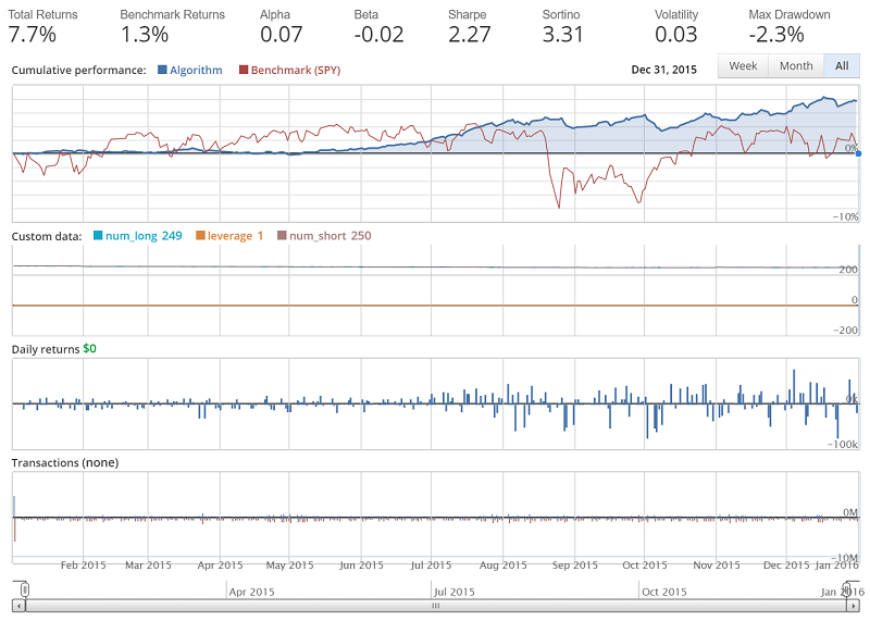
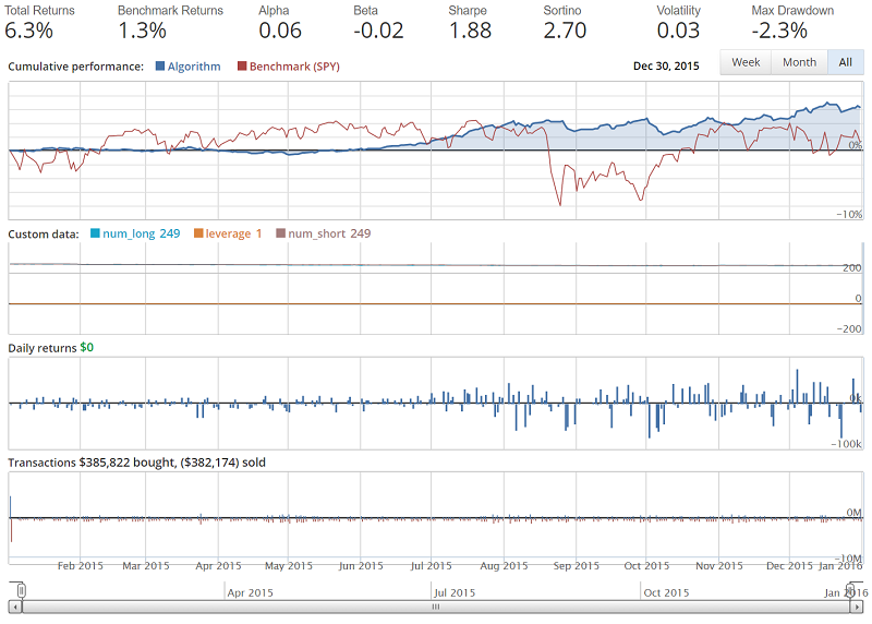
Alright, not bad. Do note that we're still including the line changing commissions: set_commission(commission.PerTrade(cost=0.001)). Even so, this strategy has already out-performed our previous strategy. You can feel free to comment that line out for the default commissions, but we're not quite yet done building our portfolio just yet. If you do comment out the commissions line, giving you default trade commissions, the result should be something like:
Let's go ahead and cover portfolio optimization now. This topic is slightly more complex, but the idea is to use convex optimization to hopefully pick the best portfolio that matches certain objectives and constraints that we set. Objectives and constraints can be anything you want, but generally an objective is somewhat unbounded, and the goal is to maximize or minimize it, and a constraint is often more of a fixed value. It doesn't have to be this way, but it usually is. For example, an objective might be to maximize the Sharpe Ratio, and a constraint on this maximization objective could be that we must keep leverage to 1.0. Convex optimization can be done in Python with libraries like cvxpy and CVXOPT, but Quantopian just recently announced their Optimize API for notebooks and the Optimize API for algorithms. While convex optimization can be used for many purposes, I think we're best suited to use it in the algorithm for portfolio management. We can actually let the optimize API handle our portfolio completely. To do this, we can first clone the example from the Optimize API for algorithms, and we'll make a few modifications, giving us:
import pandas as pd

import quantopian.algorithm as algo
import quantopian.experimental.optimize as opt

from quantopian.pipeline import Pipeline
from quantopian.pipeline.data import builtin, morningstar as mstar
from quantopian.pipeline.factors import AverageDollarVolume
from quantopian.pipeline.factors.morningstar import MarketCap
from quantopian.pipeline.classifiers.morningstar import Sector

from quantopian.pipeline.data.sentdex import sentiment
from quantopian.pipeline.data.morningstar import operation_ratios
from quantopian.pipeline.filters.morningstar import Q1500US

# Algorithm Parameters
# --------------------
# Universe Selection Parameters
UNIVERSE_SIZE = 500
MIN_MARKET_CAP_PERCENTILE = 50
LIQUIDITY_LOOKBACK_LENGTH = 100

# Constraint Parameters
MAX_GROSS_LEVERAGE = 1.0
MAX_SHORT_POSITION_SIZE = 0.002  # 1.5%
MAX_LONG_POSITION_SIZE = 0.002   # 1.5%

# Scheduling Parameters
MINUTES_AFTER_OPEN_TO_TRADE = 10
BASE_UNIVERSE_RECALCULATE_FREQUENCY = 'month_start'  # {week,quarter,year}_start are also valid


def initialize(context):
    testing_factor1 = operation_ratios.operation_margin.latest
    testing_factor2 = operation_ratios.revenue_growth.latest
    testing_factor3 = sentiment.sentiment_signal.latest

    universe = (Q1500US() &
               testing_factor1.notnull() &
               testing_factor2.notnull() &
               testing_factor3.notnull())

    testing_factor1 = testing_factor1.rank(mask=universe, method='average')
    testing_factor2 = testing_factor2.rank(mask=universe, method='average')
    testing_factor3 = testing_factor3.rank(mask=universe, method='average')

    combined_alpha = testing_factor1 + testing_factor2 + testing_factor3

    # Schedule Tasks
    # --------------
    # Create and register a pipeline computing our combined alpha and a sector
    # code for every stock in our universe. We'll use these values in our
    # optimization below.
    pipe = Pipeline(
        columns={
            'alpha': combined_alpha,
            'sector': Sector(),
        },
        # combined_alpha will be NaN for all stocks not in our universe,
        # but we also want to make sure that we have a sector code for everything
        # we trade.
        screen=combined_alpha.notnull() & Sector().notnull(),
    )
    algo.attach_pipeline(pipe, 'pipe')

    # Schedule a function, 'do_portfolio_construction', to run once a week
    # ten minutes after market open.
    algo.schedule_function(
        do_portfolio_construction,
        date_rule=algo.date_rules.week_start(),
        time_rule=algo.time_rules.market_open(minutes=MINUTES_AFTER_OPEN_TO_TRADE),
        half_days=False,
    )


def before_trading_start(context, data):
    # Call pipeline_output in before_trading_start so that pipeline
    # computations happen in the 5 minute timeout of BTS instead of the 1
    # minute timeout of handle_data/scheduled functions.
    context.pipeline_data = algo.pipeline_output('pipe')


# Portfolio Construction
# ----------------------
def do_portfolio_construction(context, data):
    pipeline_data = context.pipeline_data
    todays_universe = pipeline_data.index

    # Objective
    # ---------
    # For our objective, we simply use our naive ranks as an alpha coefficient
    # and try to maximize that alpha.
    #
    # This is a **very** naive model. Since our alphas are so widely spread out,
    # we should expect to always allocate the maximum amount of long/short
    # capital to assets with high/low ranks.
    #
    # A more sophisticated model would apply some re-scaling here to try to generate
    # more meaningful predictions of future returns.
    objective = opt.MaximizeAlpha(pipeline_data.alpha)

    # Constraints
    # -----------
    # Constrain our gross leverage to 1.0 or less. This means that the absolute
    # value of our long and short positions should not exceed the value of our
    # portfolio.
    constrain_gross_leverage = opt.MaxGrossLeverage(MAX_GROSS_LEVERAGE)

    # Constrain individual position size to no more than a fixed percentage
    # of our portfolio. Because our alphas are so widely distributed, we
    # should expect to end up hitting this max for every stock in our universe.
    constrain_pos_size = opt.PositionConcentration.with_equal_bounds(
        -MAX_SHORT_POSITION_SIZE,
        MAX_LONG_POSITION_SIZE,
    )

    # Constrain ourselves to allocate the same amount of capital to
    # long and short positions.
    market_neutral = opt.DollarNeutral()

    # Constrain ourselve to have a net leverage of 0.0 in each sector.
    sector_neutral = opt.NetPartitionExposure.with_equal_bounds(
        labels=pipeline_data.sector,
        min=-0.0001,
        max=0.0001,
    )

    # Run the optimization. This will calculate new portfolio weights and
    # manage moving our portfolio toward the target.
    algo.order_optimal_portfolio(
        objective=objective,
        constraints=[
            constrain_gross_leverage,
            constrain_pos_size,
            market_neutral,
            sector_neutral,
        ],
        universe=todays_universe,
    )
The result of the backtest:
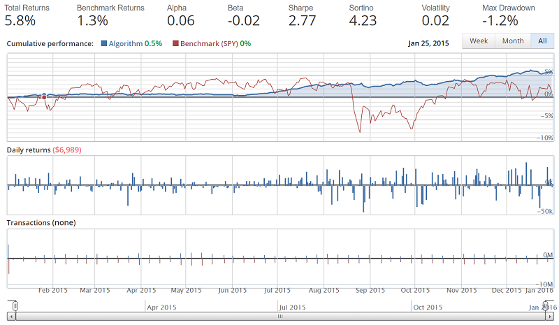
Total returns are actually a bit lower with the optimize API version, alpha and beta are the same, Sharpe is much higher for optimize, same with Sortino, Volatility is lower with optimize, and drawdown is also much less. Overall, I would have to say the decrease in volatility and drawdown is worth the slightly diminished returns, and we got that by just slapping in the Optimize API algorithm example. Lot's of possible room for improvement from here.
-
Intro and Getting Stock Price Data - Python Programming for Finance p.1
-
Handling Data and Graphing - Python Programming for Finance p.2
-
Basic stock data Manipulation - Python Programming for Finance p.3
-
More stock manipulations - Python Programming for Finance p.4
-
Automating getting the S&P 500 list - Python Programming for Finance p.5
-
Getting all company pricing data in the S&P 500 - Python Programming for Finance p.6
-
Combining all S&P 500 company prices into one DataFrame - Python Programming for Finance p.7
-
Creating massive S&P 500 company correlation table for Relationships - Python Programming for Finance p.8
-
Preprocessing data to prepare for Machine Learning with stock data - Python Programming for Finance p.9
-
Creating targets for machine learning labels - Python Programming for Finance p.10 and 11
-
Machine learning against S&P 500 company prices - Python Programming for Finance p.12
-
Testing trading strategies with Quantopian Introduction - Python Programming for Finance p.13
-
Placing a trade order with Quantopian - Python Programming for Finance p.14
-
Scheduling a function on Quantopian - Python Programming for Finance p.15
-
Quantopian Research Introduction - Python Programming for Finance p.16
-
Quantopian Pipeline - Python Programming for Finance p.17
-
Alphalens on Quantopian - Python Programming for Finance p.18
-
Back testing our Alpha Factor on Quantopian - Python Programming for Finance p.19
-
Analyzing Quantopian strategy back test results with Pyfolio - Python Programming for Finance p.20
-
Strategizing - Python Programming for Finance p.21
-
Finding more Alpha Factors - Python Programming for Finance p.22
-
Combining Alpha Factors - Python Programming for Finance p.23
-
Portfolio Optimization - Python Programming for Finance p.24
-
Zipline Local Installation for backtesting - Python Programming for Finance p.25
-
Zipline backtest visualization - Python Programming for Finance p.26
-
Custom Data with Zipline Local - Python Programming for Finance p.27
-
Custom Markets Trading Calendar with Zipline (Bitcoin/cryptocurrency example) - Python Programming for Finance p.28
