Testing NLTK and Stanford NER Taggers for Speed

Guest Post by Chuck Dishmon

We've tested our NER classifiers for accuracy, but there's more we should consider in deciding which classifier to implement. Let's test for speed next!

Just so we know we're comparing apples to apples, we'll conduct our test on the same article. Let's go with this short piece from NBC news:

House Speaker John Boehner became animated Tuesday over the proposed Keystone Pipeline, castigating the Obama administration for not having approved the project yet.

Republican House Speaker John Boehner says there's "nothing complex about the Keystone Pipeline," and that it's time to build it.

"Complex? You think the Keystone Pipeline is complex?!" Boehner responded to a questioner. "It's been under study for five years! We build pipelines in America every day. Do you realize there are 200,000 miles of pipelines in the United States?"

The speaker went on: "And the only reason the president's involved in the Keystone Pipeline is because it crosses an international boundary. Listen, we can build it. There's nothing complex about the Keystone Pipeline -- it's time to build it."

Boehner said the president had no excuse at this point to not give the pipeline the go-ahead after the State Department released a report on Friday indicating the project would have a minimal impact on the environment.

Republicans have long pushed for construction of the project, which enjoys some measure of Democratic support as well. The GOP is considering conditioning an extension of the debt limit on approval of the project by Obama.

The White House, though, has said that it has no timetable for a final decision on the project.

First we'll make our imports and process the article by reading and tokenizing.

# -*- coding: utf-8 -*-

import nltk
import os
import numpy as np
import matplotlib.pyplot as plt
from matplotlib import style
from nltk import pos_tag
from nltk.tag import StanfordNERTagger
from nltk.tokenize import word_tokenize

style.use('fivethirtyeight')

# Process text  
def process_text(txt_file):
	raw_text = open("/usr/share/news_article.txt").read()
	token_text = word_tokenize(raw_text)
	return token_text

Perfect! Now let's write some functions to separate out our classification tasks. We'll include POS tagging in our NLTK function since it's required for the NLTK NE classifier.

# Stanford NER tagger    
def stanford_tagger(token_text):
	st = StanfordNERTagger('/usr/share/stanford-ner/classifiers/english.all.3class.distsim.crf.ser.gz',
							'/usr/share/stanford-ner/stanford-ner.jar',
							encoding='utf-8')   
	ne_tagged = st.tag(token_text)
	return(ne_tagged)
 
# NLTK POS and NER taggers   
def nltk_tagger(token_text):
	tagged_words = nltk.pos_tag(token_text)
	ne_tagged = nltk.ne_chunk(tagged_words)
	return(ne_tagged)

Each classifier needs to read the article and classify the named entities, so we'll wrap these functions in a larger function to make timing easy.

def stanford_main():
	print(stanford_tagger(process_text(txt_file)))

def nltk_main():
	print(nltk_tagger(process_text(txt_file)))

Let's call the functions when we call our program. We'll wrap our stanford_main() and nltk_main() functions in os.times() functions, taking the 4th index, elapsed time. Then we'll graph our results.

if __name__ == '__main__':
	stanford_t0 = os.times()[4]
	stanford_main()
	stanford_t1 = os.times()[4]
	stanford_total_time = stanford_t1 - stanford_t0
	
	nltk_t0 = os.times()[4]
	nltk_main()
	nltk_t1 = os.times()[4]
	nltk_total_time = nltk_t1 - nltk_t0
	
	time_plot(stanford_total_time, nltk_total_time)

For our graph, we'll be using the folloing time_plot() function:

def time_plot(stanford_total_time, nltk_total_time):
	N = 1
	ind = np.arange(N)  # the x locations for the groups
	width = 0.35       # the width of the bars
	stanford_total_time = stanford_total_time
	nltk_total_time = nltk_total_time   
	fig, ax = plt.subplots()    
	rects1 = ax.bar(ind, stanford_total_time, width, color='r')    
	rects2 = ax.bar(ind+width, nltk_total_time, width, color='y')
	
	# Add text for labels, title and axes ticks
	ax.set_xlabel('Classifier')
	ax.set_ylabel('Time (in seconds)')
	ax.set_title('Speed by NER Classifier')
	ax.set_xticks(ind+width)
	ax.set_xticklabels( ('') )   
	ax.legend( (rects1[0], rects2[0]), ('Stanford', 'NLTK'), bbox_to_anchor=(1.05, 1), loc=2, borderaxespad=0. )

	def autolabel(rects):
		# attach some text labels
		for rect in rects:
			height = rect.get_height()
			ax.text(rect.get_x()+rect.get_width()/2., 1.02*height, '%10.2f' % float(height),
					ha='center', va='bottom')
	
	autolabel(rects1)
	autolabel(rects2)    
	plt.show()

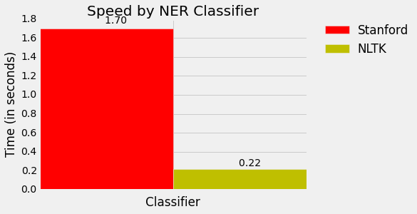
Whoa, NLTK is lightning fast! It seems Stanford is more accurate, but NLTK is faster. This is great information to know when weighing our preferred level of precision alongside required computing resources.

But wait, there's still a problem. Our output is ugly! Here's a small sample from Stanford:

[('House', 'ORGANIZATION'), ('Speaker', 'O'), ('John', 'PERSON'), ('Boehner', 'PERSON'), ('became', 'O'), ('animated', 'O'), ('Tuesday', 'O'), ('over', 'O'), ('the', 'O'), ('proposed', 'O'), ('Keystone', 'ORGANIZATION'), ('Pipeline', 'ORGANIZATION'), (',', 'O'), ('castigating', 'O'), ('the', 'O'), ('Obama', 'PERSON'), ('administration', 'O'), ('for', 'O'), ('not', 'O'), ('having', 'O'), ('approved', 'O'), ('the', 'O'), ('project', 'O'), ('yet', 'O'), ('.', 'O')

And from NLTK:

(S
  (ORGANIZATION House/NNP)
  Speaker/NNP
  (PERSON John/NNP Boehner/NNP)
  became/VBD
  animated/VBN
  Tuesday/NNP
  over/IN
  the/DT
  proposed/VBN
  (PERSON Keystone/NNP Pipeline/NNP)
  ,/,
  castigating/VBG
  the/DT
  (ORGANIZATION Obama/NNP)
  administration/NN
  for/IN
  not/RB
  having/VBG
  approved/VBN
  the/DT
  project/NN
  yet/RB
  ./.

Let's get these into nice readable forms in the next tutorial!

The next tutorial: Using BIO Tags to Create Readable Named Entity Lists