Optimizing Models with TensorBoard - Deep Learning basics with Python, TensorFlow and Keras p.5
Welcome to part 5 of the Deep learning with Python, TensorFlow and Keras tutorial series. In the previous tutorial, we introduced TensorBoard, which is an application that we can use to visualize our model's training stats over time. In this tutorial, we're going to continue on that to exemplify how you might build a workflow to optimize your model's architecture.
To begin, let's think of a few things we could do to this model that we'd like to know.
The most basic things for us to modify are layers and nodes per layer, as well as 0, 1, or 2 dense layers. Let's test those things. How might we do this?
A simple for-loop will do! For example:
import time

dense_layers = [0,1,2]
layer_sizes = [32, 64, 128]
conv_layers = [1, 2, 3]

for dense_layer in dense_layers:
    for layer_size in layer_sizes:
        for conv_layer in conv_layers:
            NAME = "{}-conv-{}-nodes-{}-dense-{}".format(conv_layer, layer_size, dense_layer, int(time.time()))
            print(NAME)
So that's a lot of combinations. I will be running them all, you don't have to. If you have a decent GPU, you can install and use Tensorflow-GPU instead. If you want to learn how to do that, I have two tutorials doing it:
Both videos are for an older version of TF, but the methodology for getting Tensorflow-GPU is fairly straight forward. You do a pip install tensorflow-gpu, then download the Cuda Toolkit, and then CuDNN. Install Cuda Toolkit, and copy the files over from CuDNN to the toolkit. Check out the videos above for more help on this, however. Also make sure you grab the right versions of Cuda Toolkit and CuDNN. See the installation docs on Tensorflow.org for your operating system to get the version #s you need!
You can also use GPUs in the cloud. I recommend Paperspace for this, and I covered using them in this video
Anywho, let's build the model next.
dense_layers = [0, 1, 2]
layer_sizes = [32, 64, 128]
conv_layers = [1, 2, 3]

for dense_layer in dense_layers:
    for layer_size in layer_sizes:
        for conv_layer in conv_layers:
            NAME = "{}-conv-{}-nodes-{}-dense-{}".format(conv_layer, layer_size, dense_layer, int(time.time()))
            print(NAME)

            model = Sequential()

            model.add(Conv2D(layer_size, (3, 3), input_shape=X.shape[1:]))
            model.add(Activation('relu'))
            model.add(MaxPooling2D(pool_size=(2, 2)))

            for l in range(conv_layer-1):
                model.add(Conv2D(layer_size, (3, 3)))
                model.add(Activation('relu'))
                model.add(MaxPooling2D(pool_size=(2, 2)))

            model.add(Flatten())
            for _ in range(dense_layer):
                model.add(Dense(layer_size))
                model.add(Activation('relu'))

            model.add(Dense(1))
            model.add(Activation('sigmoid'))
Even just toying with these parameters will take some significant time. We haven't even begun to touch other concepts like varying layer sizes, activation functions, learning rates, dropouts, and much much more.
In general, I try to test only a few things. You almost want to make a hill-climb operation out of this process. First find a model that works. On this dataset, that part was easy. Then try to tinker with 2 or 3 things max. If there's a long/infinite list of options, such as is the case with layer count and nodes per layer, try to just do maybe one move in each direction.
For example, if you find a 64 node-per-layer is working. Try a 32 and a 128, along with 64, so your list is [32, 64, 128]. If 128 shows better results, then maybe try [64, 128, 256] next, and so on.
Just note that, as you change certain parameters, you may need to revisit older ones. As you tweak dropout, for example, let's say you add or just increase dropout. As you add or increase dropout, you can likely have a larger overall model in terms of layers or nodes per layer than before. A larger model overall might want a larger starting learning rate or a slower rate of decay for the learning rate.
Finally, take note that there is some randomness in models. No two rounds of optimizations will be identical. They should be close, but not identical. Models are also initialized with random weights. This can impact models fairly significantly, especially in shorter numbers of epochs or if you have a small training set.
Anyway, here's the full script for initial model testing:
from tensorflow.keras.models import Sequential
from tensorflow.keras.layers import Dense, Dropout, Activation, Flatten
from tensorflow.keras.layers import Conv2D, MaxPooling2D
# more info on callbakcs: https://keras.io/callbacks/ model saver is cool too.
from tensorflow.keras.callbacks import TensorBoard
import pickle
import time

pickle_in = open("X.pickle","rb")
X = pickle.load(pickle_in)

pickle_in = open("y.pickle","rb")
y = pickle.load(pickle_in)

X = X/255.0

dense_layers = [0, 1, 2]
layer_sizes = [32, 64, 128]
conv_layers = [1, 2, 3]

for dense_layer in dense_layers:
    for layer_size in layer_sizes:
        for conv_layer in conv_layers:
            NAME = "{}-conv-{}-nodes-{}-dense-{}".format(conv_layer, layer_size, dense_layer, int(time.time()))
            print(NAME)

            model = Sequential()

            model.add(Conv2D(layer_size, (3, 3), input_shape=X.shape[1:]))
            model.add(Activation('relu'))
            model.add(MaxPooling2D(pool_size=(2, 2)))

            for l in range(conv_layer-1):
                model.add(Conv2D(layer_size, (3, 3)))
                model.add(Activation('relu'))
                model.add(MaxPooling2D(pool_size=(2, 2)))

            model.add(Flatten())

            for _ in range(dense_layer):
                model.add(Dense(layer_size))
                model.add(Activation('relu'))

            model.add(Dense(1))
            model.add(Activation('sigmoid'))

            tensorboard = TensorBoard(log_dir="logs/{}".format(NAME))

            model.compile(loss='binary_crossentropy',
                          optimizer='adam',
                          metrics=['accuracy'],
                          )

            model.fit(X, y,
                      batch_size=32,
                      epochs=10,
                      validation_split=0.3,
                      callbacks=[tensorboard])
Results for this:
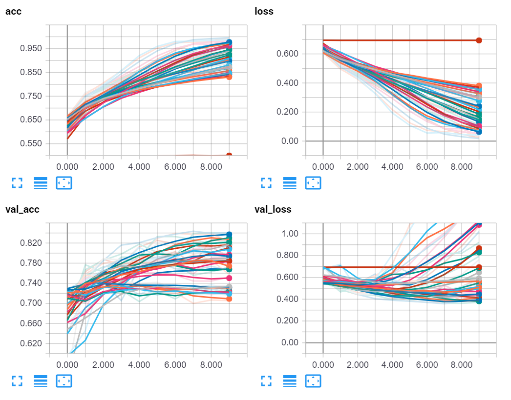
It could be tempting to take the highest validation accuracy model, but I tend to instead go for the best (lowest) validation loss models. Like I said before, there is some randomness when it comes to models, but you should notice trends.
For one, I notice that the models with 0 dense layers seemed to do better overall. There are some very successful models with dense layers, but I am going to guess one is likely not needed here.
So, zooming into the validation accuracy graph, let's check some of the best ones. Here are the top 10:
- 3 conv, 64 nodes per layer, 0 dense
- 3 conv, 128 nodes per layer, 0 dense
- 3 conv, 32 nodes per layer, 0 dense
- 3 conv, 32 nodes per layer, 2 dense
- 3 conv, 32 nodes per layer, 1 dense
- 2 conv, 32 nodes per layer, 0 dense
- 2 conv, 64 nodes per layer, 0 dense
- 3 conv, 128 nodes per layer, 1 dense
- 2 conv, 128 nodes per layer, 0 dense
- 2 conv, 32 nodes per layer, 1 dense
From here, I think we can be comfortable with 0 dense, and 3 convolutional layers, since every version of those 2 options proved to be better than anything else. Just the top 3 models:
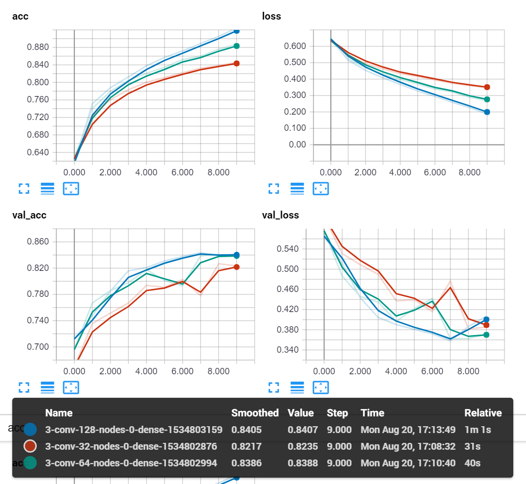
-
Introduction to Deep Learning - Deep Learning basics with Python, TensorFlow and Keras p.1
-
Loading in your own data - Deep Learning basics with Python, TensorFlow and Keras p.2
-
Convolutional Neural Networks - Deep Learning basics with Python, TensorFlow and Keras p.3
-
Analyzing Models with TensorBoard - Deep Learning basics with Python, TensorFlow and Keras p.4
-
Optimizing Models with TensorBoard - Deep Learning basics with Python, TensorFlow and Keras p.5
-
How to use your trained model - Deep Learning basics with Python, TensorFlow and Keras p.6
-
Recurrent Neural Networks - Deep Learning basics with Python, TensorFlow and Keras p.7
-
Creating a Cryptocurrency-predicting finance recurrent neural network - Deep Learning basics with Python, TensorFlow and Keras p.8
-
Normalizing and creating sequences for our cryptocurrency predicting RNN - Deep Learning basics with Python, TensorFlow and Keras p.9
-
Balancing Recurrent Neural Network sequence data for our crypto predicting RNN - Deep Learning basics with Python, TensorFlow and Keras p.10
-
Cryptocurrency-predicting RNN Model - Deep Learning basics with Python, TensorFlow and Keras p.11
