Analyzing Models with TensorBoard - Deep Learning basics with Python, TensorFlow and Keras p.4
Welcome to part 4 of the deep learning basics with Python, TensorFlow, and Keras tutorial series. In this part, what we're going to be talking about is TensorBoard. TensorBoard is a handy application that allows you to view aspects of your model, or models, in your browser.
The way that we use TensorBoard with Keras is via a Keras callback. There are actually quite a few Keras callbacks, and you can make your own. Definitely check the others out: Keras Callbacks. For example, ModelCheckpoint is another useful one. For now, however, we're going to be focused on the TensorBoard callback. We
To begin, we need to add the following to our imports:
from tensorflow.keras.callbacks import TensorBoard
Now we want to make our TensorBoard callback object:
NAME = "Cats-vs-dogs-CNN"

tensorboard = TensorBoard(log_dir="logs/{}".format(NAME))
Eventually, you will want to get a little more custom with your NAME, but this will do for now. So this will save the model's training data to logs/NAME, which can then be read by TensorBoard.
Finally, we can add this callback to our model by adding it to the .fit method, like:
model.fit(X, y,
          batch_size=32,
          epochs=3,
          validation_split=0.3,
          callbacks=[tensorboard])
Notice that callbacks is a list. You can pass other callbacks into this list as well. Our model isn't defined yet, so let's put this all together now:
import tensorflow as tf
from tensorflow.keras.datasets import cifar10
from tensorflow.keras.preprocessing.image import ImageDataGenerator
from tensorflow.keras.models import Sequential
from tensorflow.keras.layers import Dense, Dropout, Activation, Flatten
from tensorflow.keras.layers import Conv2D, MaxPooling2D
# more info on callbakcs: https://keras.io/callbacks/ model saver is cool too.
from tensorflow.keras.callbacks import TensorBoard
import pickle
import time

NAME = "Cats-vs-dogs-CNN"

pickle_in = open("X.pickle","rb")
X = pickle.load(pickle_in)

pickle_in = open("y.pickle","rb")
y = pickle.load(pickle_in)

X = X/255.0

model = Sequential()

model.add(Conv2D(256, (3, 3), input_shape=X.shape[1:]))
model.add(Activation('relu'))
model.add(MaxPooling2D(pool_size=(2, 2)))

model.add(Conv2D(256, (3, 3)))
model.add(Activation('relu'))
model.add(MaxPooling2D(pool_size=(2, 2)))

model.add(Flatten())  # this converts our 3D feature maps to 1D feature vectors
model.add(Dense(64))

model.add(Dense(1))
model.add(Activation('sigmoid'))

tensorboard = TensorBoard(log_dir="logs/{}".format(NAME))

model.compile(loss='binary_crossentropy',
              optimizer='adam',
              metrics=['accuracy'],
              )

model.fit(X, y,
          batch_size=32,
          epochs=3,
          validation_split=0.3,
          callbacks=[tensorboard])
After having run this, you should have a new directory called logs. We can visualize the initial results from this directory using tensorboard now. Open a console, change to your working directory, and type: tensorboard --logdir=logs/. You should see a notice like: TensorBoard 1.10.0 at http://H-PC:6006 (Press CTRL+C to quit) where "h-pc" probably is whatever your machine's name is. Open a browser and head to this address. You should see something like:
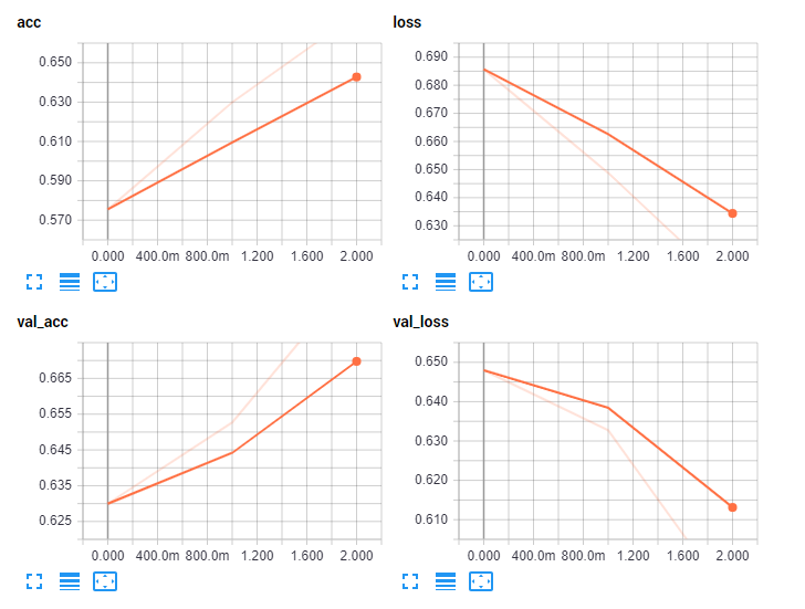
Now we can see how our model did over time. Let's change some things in our model. To begin, we never added an activation to our dense layer. Also, let's try a smaller model overall:
from tensorflow.keras.models import Sequential
from tensorflow.keras.layers import Dense, Dropout, Activation, Flatten
from tensorflow.keras.layers import Conv2D, MaxPooling2D
# more info on callbakcs: https://keras.io/callbacks/ model saver is cool too.
from tensorflow.keras.callbacks import TensorBoard
import pickle
import time

NAME = "Cats-vs-dogs-64x2-CNN"

pickle_in = open("X.pickle","rb")
X = pickle.load(pickle_in)

pickle_in = open("y.pickle","rb")
y = pickle.load(pickle_in)

X = X/255.0

model = Sequential()

model.add(Conv2D(64, (3, 3), input_shape=X.shape[1:]))
model.add(Activation('relu'))
model.add(MaxPooling2D(pool_size=(2, 2)))

model.add(Conv2D(64, (3, 3)))
model.add(Activation('relu'))
model.add(MaxPooling2D(pool_size=(2, 2)))

model.add(Flatten())  # this converts our 3D feature maps to 1D feature vectors
model.add(Dense(64))
model.add(Activation('relu'))

model.add(Dense(1))
model.add(Activation('sigmoid'))

tensorboard = TensorBoard(log_dir="logs/{}".format(NAME))

model.compile(loss='binary_crossentropy',
              optimizer='adam',
              metrics=['accuracy'],
              )

model.fit(X, y,
          batch_size=32,
          epochs=10,
          validation_split=0.3,
          callbacks=[tensorboard])
Among other things, I also changed the name to NAME = "Cats-vs-dogs-64x2-CNN". Don't forget to do this, or you'll append to your previous model's logs instead by accident and it wont look too good. Let's check TensorBoard now:
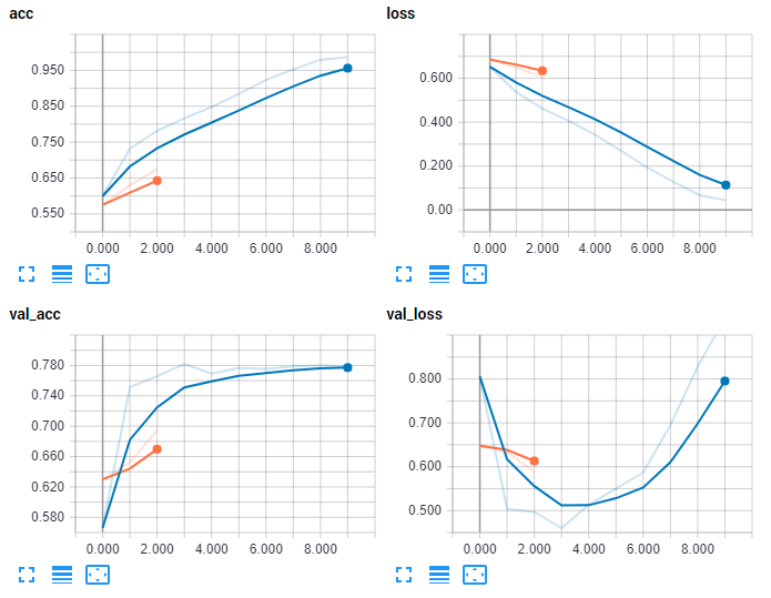
Looking better! Immediately, however, you might notice the shape of validation loss. Loss is the measure of error, and it clearly looks like, after our 4th epoch, things began to sour. Interestingly enough, our validation accuracy still continued to hold, but I imagine it would eventually begin to fall. It's much more likely that the first thing to suffer will indeed be your validation loss. This should alert you that you're almost certainly beginning to over-fit. The reason why this happens is the model is constantly trying to decrease your in-sample loss. At some point, rather than learning general things about the actual data, the model instead begins to just memorize input data. If you let this continue, yes your "accuracy" in-sample will rise, but your out of sample, and any new data you attempt to feed the model, will perform poorly.
In the next tutorial, we'll talk about how you can use TensorBoard to optimize the model you use with your data.
-
Introduction to Deep Learning - Deep Learning basics with Python, TensorFlow and Keras p.1
-
Loading in your own data - Deep Learning basics with Python, TensorFlow and Keras p.2
-
Convolutional Neural Networks - Deep Learning basics with Python, TensorFlow and Keras p.3
-
Analyzing Models with TensorBoard - Deep Learning basics with Python, TensorFlow and Keras p.4
-
Optimizing Models with TensorBoard - Deep Learning basics with Python, TensorFlow and Keras p.5
-
How to use your trained model - Deep Learning basics with Python, TensorFlow and Keras p.6
-
Recurrent Neural Networks - Deep Learning basics with Python, TensorFlow and Keras p.7
-
Creating a Cryptocurrency-predicting finance recurrent neural network - Deep Learning basics with Python, TensorFlow and Keras p.8
-
Normalizing and creating sequences for our cryptocurrency predicting RNN - Deep Learning basics with Python, TensorFlow and Keras p.9
-
Balancing Recurrent Neural Network sequence data for our crypto predicting RNN - Deep Learning basics with Python, TensorFlow and Keras p.10
-
Cryptocurrency-predicting RNN Model - Deep Learning basics with Python, TensorFlow and Keras p.11
