Linear SVC machine learning and testing our data

In this video, we're going to cover using two features for machine learning, using Linear SVC with our data. We have many more features to add as time goes on, but we want to use two features at first so that we can easily visualize our data.

import numpy as np
import matplotlib.pyplot as plt
from sklearn import svm
import pandas as pd
from matplotlib import style
style.use("ggplot")

Typical imports above, all of which have been explained up to this point.

Next, we want to have a function that can build a data-set in a way that is understandable for Scikit-learn.

def Build_Data_Set(features = ["DE Ratio",
                               "Trailing P/E"]):
    data_df = pd.DataFrame.from_csv("key_stats.csv")

    data_df = data_df[:100]

    X = np.array(data_df[features].values)

    y = (data_df["Status"]
         .replace("underperform",0)
         .replace("outperform",1)
         .values.tolist())


    return X,y

In this function, we specify two default parameters, though we could add more when we call the function. Then we call upon the key_stats.csv file to be loaded into data_df. From there, we chop this to only include the first 100 rows of data.

Next, we fill the X parameter with the NumPy array containing rows of features. After this, we're going to populate the y variable with the "targets," or "labels," converted to numerical data.

Finally, we return the X, and y variable to be unpacked. Now we're going to define an analysis function.

def Analysis():
    X, y = Build_Data_Set()

    clf = svm.SVC(kernel="linear", C= 1.0)
    clf.fit(X,y)
    
    w = clf.coef_[0]
    a = -w[0] / w[1]
    xx = np.linspace(min(X[:, 0]), max(X[:, 0]))
    yy = a * xx - clf.intercept_[0] / w[1]

    h0 = plt.plot(xx,yy, "k-", label="non weighted")

    plt.scatter(X[:, 0],X[:, 1],c=y)
    plt.ylabel("Trailing P/E")
    plt.xlabel("DE Ratio")
    plt.legend()

    plt.show()
    
Analysis()

The above code should all be familiar to anyone following along in order. If you still have questions, however, you can feel free to comment below or on the YouTube video.

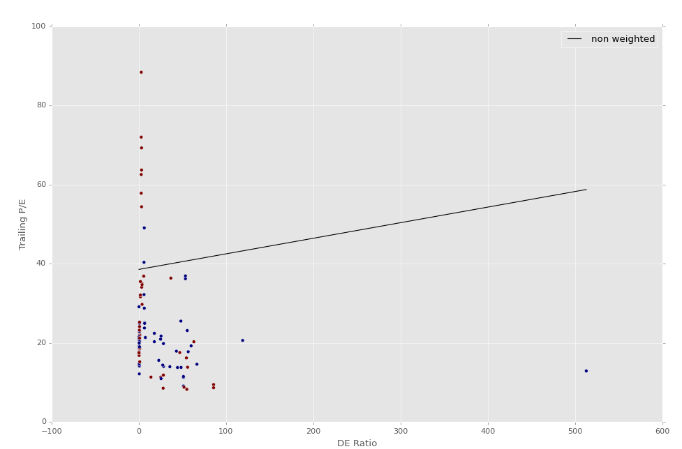
The following graph should be similar to your output. Just in case something is wrong with your Key_Stats.csv file, here's my file for S&P 500 company fundamental statistics:

Looking at this image, it doesn't appear that there is anything of value, other than that water is wet. If we look, we can see we have some red, and some blue dots. The red dots are the out-performers and the blue dots are under-performers.

Some people may point out that it looks like there is a clear divide that seemingly separates a group of mostly out-performing feature sets. Let's analyze the features used in this example.

First, Debt/Equity. We can see here pretty clearly that out-performing stocks, at least in our small, sliced example, appear to be stocks that have low Debt/Equity. That's somewhat useful (though not as useful looking at today's companies), also even further un-useful for reasons discussed later (using the first 100 rows uses on the first 100 data files, meaning we probably are not even getting out of the companies that start with the letter A here).

The other feature being used here is Trailing P/E, which is trailing price to earnings. Trailing, meaning according to older values. So what is the price, today, in accordance with earnings from the past, usually 12 months.

It only stands to reason that companies outperforming today are companies with a high current price compared to their previous earnings, as outperforming the market suggests price has indeed been rising.

With these issues in mind, we know we have some work ahead of us.

The next tutorial: Scaling, Normalizing, and machine learning with many features