Convolutional Neural Networks - Deep Learning basics with Python, TensorFlow and Keras p.3
Welcome to a tutorial where we'll be discussing Convolutional Neural Networks (Convnets and CNNs), using one to classify dogs and cats with the dataset we built in the previous tutorial.
The Convolutional Neural Network gained popularity through its use with image data, and is currently the state of the art for detecting what an image is, or what is contained in the image.
The basic CNN structure is as follows: Convolution -> Pooling -> Convolution -> Pooling -> Fully Connected Layer -> Output
Convolution is the act of taking the original data, and creating feature maps from it.Pooling is down-sampling, most often in the form of "max-pooling," where we select a region, and then take the maximum value in that region, and that becomes the new value for the entire region. Fully Connected Layers are typical neural networks, where all nodes are "fully connected." The convolutional layers are not fully connected like a traditional neural network.
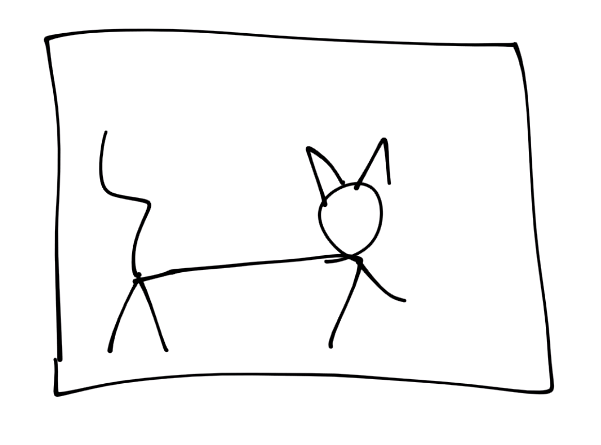
Okay, so now let's depict what's happening. We'll start with an image of a cat:
Then "convert to pixels:"
![]()
For the purposes of this tutorial, assume each square is a pixel. Next, for the convolution step, we're going to take a certain window, and find features within that window:
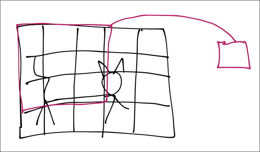
That window's features are now just a single pixel-sized feature in a new featuremap, but we will have multiple layers of featuremaps in reality.
Next, we slide that window over and continue the process. There will be some overlap, you can determine how much you want, you just do not want to be skipping any pixels, of course.
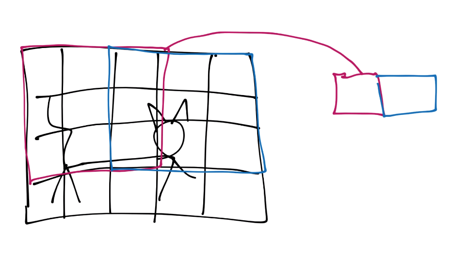
Now you continue this process until you've covered the entire image, and then you will have a featuremap. Typically the featuremap is just more pixel values, just a very simplified one:
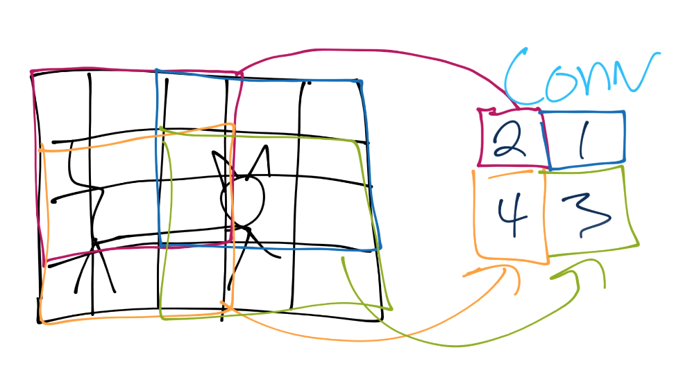
From here, we do pooling. Let's say our convolution gave us (I forgot to put a number in the 2nd row's most right square, assume it's a 3 or less):
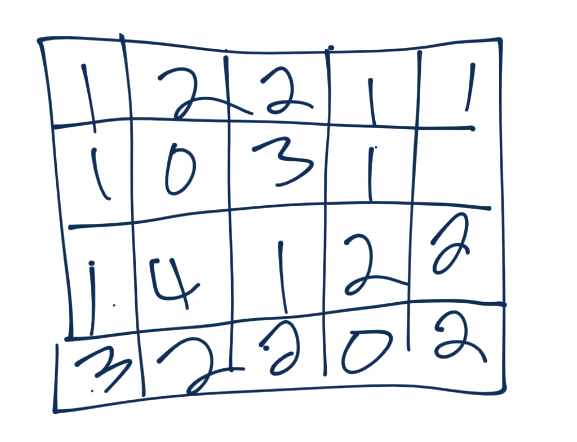
Now we'll take a 3x3 pooling window:
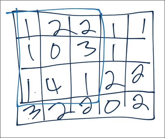
The most common form of pooling is "max pooling," where we simple take the maximum value in the window, and that becomes the new value for that region.
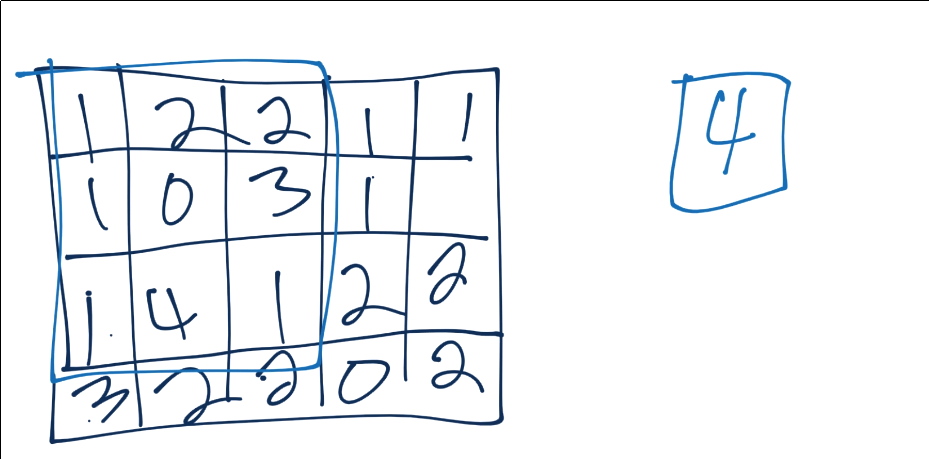
We continue this process, until we've pooled, and have something like:
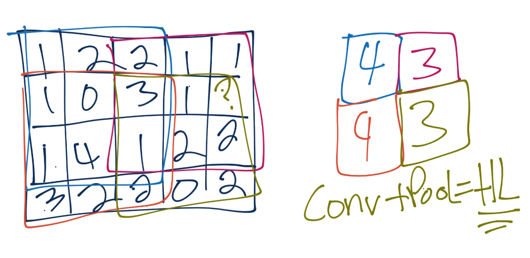
Each convolution and pooling step is a hidden layer. After this, we have a fully connected layer, followed by the output layer. The fully connected layer is your typical neural network (multilayer perceptron) type of layer, and same with the output layer.
import tensorflow as tf
from tensorflow.keras.datasets import cifar10
from tensorflow.keras.preprocessing.image import ImageDataGenerator
from tensorflow.keras.models import Sequential
from tensorflow.keras.layers import Dense, Dropout, Activation, Flatten
from tensorflow.keras.layers import Conv2D, MaxPooling2D

import pickle

pickle_in = open("X.pickle","rb")
X = pickle.load(pickle_in)

pickle_in = open("y.pickle","rb")
y = pickle.load(pickle_in)

X = X/255.0

model = Sequential()

model.add(Conv2D(256, (3, 3), input_shape=X.shape[1:]))
model.add(Activation('relu'))
model.add(MaxPooling2D(pool_size=(2, 2)))

model.add(Conv2D(256, (3, 3)))
model.add(Activation('relu'))
model.add(MaxPooling2D(pool_size=(2, 2)))

model.add(Flatten())  # this converts our 3D feature maps to 1D feature vectors

model.add(Dense(64))

model.add(Dense(1))
model.add(Activation('sigmoid'))

model.compile(loss='binary_crossentropy',
              optimizer='adam',
              metrics=['accuracy'])

model.fit(X, y, batch_size=32, epochs=3, validation_split=0.3)
After just three epochs, we have 71% validation accuracy. If we keep going, we can probably do even better, but we should probably discuss how we know how we are doing. To help with this, we can use TensorBoard, which comes with TensorFlow and it helps you visualize your models as they are trained.
We'll talk about TensorBoard as well as various tweaks to our model in the next tutorial!
-
Introduction to Deep Learning - Deep Learning basics with Python, TensorFlow and Keras p.1
-
Loading in your own data - Deep Learning basics with Python, TensorFlow and Keras p.2
-
Convolutional Neural Networks - Deep Learning basics with Python, TensorFlow and Keras p.3
-
Analyzing Models with TensorBoard - Deep Learning basics with Python, TensorFlow and Keras p.4
-
Optimizing Models with TensorBoard - Deep Learning basics with Python, TensorFlow and Keras p.5
-
How to use your trained model - Deep Learning basics with Python, TensorFlow and Keras p.6
-
Recurrent Neural Networks - Deep Learning basics with Python, TensorFlow and Keras p.7
-
Creating a Cryptocurrency-predicting finance recurrent neural network - Deep Learning basics with Python, TensorFlow and Keras p.8
-
Normalizing and creating sequences for our cryptocurrency predicting RNN - Deep Learning basics with Python, TensorFlow and Keras p.9
-
Balancing Recurrent Neural Network sequence data for our crypto predicting RNN - Deep Learning basics with Python, TensorFlow and Keras p.10
-
Cryptocurrency-predicting RNN Model - Deep Learning basics with Python, TensorFlow and Keras p.11
