Resampling - p.9 Data Analysis with Python and Pandas Tutorial

Welcome to another data analysis with Python and Pandas tutorial. In this tutorial, we're going to be talking about smoothing out data by removing noise. There are two main methods to do this. The most popular method used is what is called resampling, though it might take many other names. This is where we have some data that is sampled at a certain rate. For us, we have the Housing Price Index sampled at a one-month rate, but we could sample the HPI every week, every day, every minute, or more, but we could also resample at every year, every 10 years, and so on.

Another environment where resampling almost always occurs is with stock prices, for example. Stock prices are intra-second. What winds up happening though, is usually stock prices are resampled to minute data at the lowest for free data. You can buy access to live data, however. On a long-term scale, usually the data will be sampled daily, or even every 3-5 days. This is often done to keep the size of the data being transferred low. For example, over the course of, say, one year, intra-second data is usually in the multiples of gigabytes, and transferring all of that at once is unreasonable and people would be waiting minutes or hours for pages to load.

Using our current data, which is currently sampled at once a month, how might we sample it instead to once every 6 months, or 2 years? Try to think about how you might personally write a function that might perform that task, it's a fairly challenging one, but it can be done. That said, it's a fairly computationally inefficient job, but Pandas has our backs and does it very fast. Let's see. Our starting script right now:

import Quandl
import pandas as pd
import pickle
import matplotlib.pyplot as plt
from matplotlib import style
style.use('fivethirtyeight')

# Not necessary, I just do this so I do not show my API key.
api_key = open('quandlapikey.txt','r').read()

def state_list():
    fiddy_states = pd.read_html('https://simple.wikipedia.org/wiki/List_of_U.S._states')
    return fiddy_states[0][0][1:]
    

def grab_initial_state_data():
    states = state_list()

    main_df = pd.DataFrame()

    for abbv in states:
        query = "FMAC/HPI_"+str(abbv)
        df = Quandl.get(query, authtoken=api_key)
        print(query)
        df[abbv] = (df[abbv]-df[abbv][0]) / df[abbv][0] * 100.0
        print(df.head())
        if main_df.empty:
            main_df = df
        else:
            main_df = main_df.join(df)
            
    pickle_out = open('fiddy_states3.pickle','wb')
    pickle.dump(main_df, pickle_out)
    pickle_out.close()

def HPI_Benchmark():
    df = Quandl.get("FMAC/HPI_USA", authtoken=api_key)
    df["United States"] = (df["United States"]-df["United States"][0]) / df["United States"][0] * 100.0
    return df
fig = plt.figure()
ax1 = plt.subplot2grid((1,1), (0,0))
HPI_data = pd.read_pickle('fiddy_states3.pickle')
HPI_State_Correlation = HPI_data.corr()

First, let's make this a bit more basic, and just reference the Texas information first, but also resample it:

TX1yr = HPI_data['TX'].resample('A')
print(TX1yr.head())

Output:

Date
1975-12-31     4.559105
1976-12-31    11.954152
1977-12-31    23.518179
1978-12-31    41.978042
1979-12-31    64.700665
Freq: A-DEC, Name: TX, dtype: float64

We resampled with the "A," which resamples annually (year-end). You can find all of the resample options here: http://pandas.pydata.org/pandas-docs/stable/timeseries.html#offset-aliases, but here are the current ones as of my writing this tutorial:

Resample rule:
xL for milliseconds
xMin for minutes
xD for Days

Alias	Description
B	business day frequency
C	custom business day frequency (experimental)
D	calendar day frequency
W	weekly frequency
M	month end frequency
BM	business month end frequency
CBM	custom business month end frequency
MS	month start frequency
BMS	business month start frequency
CBMS	custom business month start frequency
Q	quarter end frequency
BQ	business quarter endfrequency
QS	quarter start frequency
BQS	business quarter start frequency
A	year end frequency
BA	business year end frequency
AS	year start frequency
BAS	business year start frequency
BH	business hour frequency
H	hourly frequency
T	minutely frequency
S	secondly frequency
L	milliseonds
U	microseconds
N	nanoseconds

How:
mean, sum, ohlc

Now we can compare the two data sets:

HPI_data['TX'].plot(ax=ax1)
TX1yr.plot(color='k',ax=ax1)

plt.legend().remove()
plt.show()

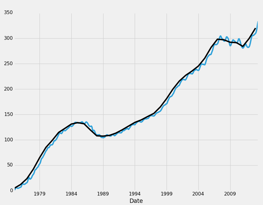
As you can see, moving from monthly to annual data has not really hidden anything from us regarding the trend line itself, but one interesting thing to note, however, at least here for Texas, do you think those wiggles in the monthly data look a bit patterned? I do. You can hover your mouse over all the peaks, and start looking at the month out of the year that these peaks are occuring. Most of the peaks are occuring around 6 months in, with just about every low occuring around December. A lot of states have this pattern, and it comes through in the US HPI. Maybe we will just play those trends and be done with the entire tutorial! We are now experts!

Okay not really, I guess we'll continue on with the tutorial. So with resampling, we can choose the interval, as well as "how" we wish to resample. The default is by mean, but there's also a sum of that period. If we resampled by year, with how=sum, then the return would be a sum of all the HPI values in that 1 year. Finally, there's OHLC, which is open high low and close. This returns the starting value, the highest value, the lowest value, and the last value in that period.

I think we're better off sticking with the monthly data, but resampling is definitely worth covering in any Pandas tutorial. Now, you may be wondering why we made a new dataframe for the resampling rather than just adding it to our existing dataframe. The reason for this is it would have created a large amount of NaN data. Sometimes, even just the original resampling will contain NaN data, especially if your data is not updated by uniform intervals. Handling missing data is a major topic, but we'll attempt to cover it broadly in the next tutorial, both with the philosophy of handling missing data as well as how to handle your choices via your program.

There exists 1 challenge(s) for this tutorial. Sign up to +=1 for access to these, video downloads, and no ads.

The next tutorial: Handling Missing Data - p.10 Data Analysis with Python and Pandas Tutorial