Handling Missing Data - p.10 Data Analysis with Python and Pandas Tutorial
Welcome to Part 10 of our Data Analysis with Python and Pandas tutorial. In this part, we're going to be talking about missing or not available data. We have a few options when considering the existence of missing data.
- Ignore it - Just leave it there
- Delete it - Remove all cases. Remove from data entirely. This means forfeiting the entire row of data.
- Fill forward or backwards - This means taking the prior or following value and just filling it in.
- Replace it with something static - For example, replacing all NaN data with -9999.
Each of these options has their own merits for a variety of reasons. Ignoring it requires no more work on our end. You may choose to ignore missing data for legal reasons, or maybe to retain the utmost integrity of the data. Missing data might also be very important data. For example, maybe part of your analysis is investigating signal drops from a server. In this case, maybe the missing data is super important to keep in the set.
Next, we have delete it. You have another two choices at this point. You can either delete rows if they contain any amount of NaN data, or you can delete the row if it is completely NaN data. Usually a row that is full of NaN data comes from a calculation you performed on the dataset, and no data is really missing, it's just simply not available given your formula. In most cases, you would at least want to drop all rows that are completely NaN, and in many cases you would like to just drop rows that have any NaN data. How might we go about doing this? We'll start with the following script (notice the resampling is being done now by adding a new column to the HPI_data dataframe.):
import Quandl
import pandas as pd
import pickle
import matplotlib.pyplot as plt
from matplotlib import style
style.use('fivethirtyeight')

# Not necessary, I just do this so I do not show my API key.
api_key = open('quandlapikey.txt','r').read()

def state_list():
    fiddy_states = pd.read_html('https://simple.wikipedia.org/wiki/List_of_U.S._states')
    return fiddy_states[0][0][1:]


def grab_initial_state_data():
    states = state_list()

    main_df = pd.DataFrame()

    for abbv in states:
        query = "FMAC/HPI_"+str(abbv)
        df = Quandl.get(query, authtoken=api_key)
        print(query)
        df[abbv] = (df[abbv]-df[abbv][0]) / df[abbv][0] * 100.0
        print(df.head())
        if main_df.empty:
            main_df = df
        else:
            main_df = main_df.join(df)

    pickle_out = open('fiddy_states3.pickle','wb')
    pickle.dump(main_df, pickle_out)
    pickle_out.close()

def HPI_Benchmark():
    df = Quandl.get("FMAC/HPI_USA", authtoken=api_key)
    df["United States"] = (df["United States"]-df["United States"][0]) / df["United States"][0] * 100.0
    return df

##fig = plt.figure()
##ax1 = plt.subplot2grid((1,1), (0,0))

HPI_data = pd.read_pickle('fiddy_states3.pickle')
HPI_data['TX1yr'] = HPI_data['TX'].resample('A')
print(HPI_data[['TX','TX1yr']])

##HPI_data['TX'].plot(ax=ax1)
##HPI_data['TX1yr'].plot(color='k',ax=ax1)
##
##plt.legend().remove()
##plt.show()
We're commenting out the graphing stuff for now, but we'll revisit in a moment.
Output:
                    TX       TX1yr
Date
1975-01-31    0.000000         NaN
1975-02-28    1.291954         NaN
1975-03-31    3.348154         NaN
1975-04-30    6.097700         NaN
1975-05-31    6.887769         NaN
1975-06-30    5.566434         NaN
1975-07-31    4.710613         NaN
1975-08-31    4.612650         NaN
1975-09-30    4.831876         NaN
1975-10-31    5.192504         NaN
1975-11-30    5.832832         NaN
1975-12-31    6.336776    4.559105
1976-01-31    6.576975         NaN
1976-02-29    7.364782         NaN
1976-03-31    9.579950         NaN
1976-04-30   12.867197         NaN
1976-05-31   14.018165         NaN
1976-06-30   12.938501         NaN
1976-07-31   12.397848         NaN
1976-08-31   12.388581         NaN
1976-09-30   12.638779         NaN
1976-10-31   13.341849         NaN
1976-11-30   14.336404         NaN
1976-12-31   15.000798   11.954152
1977-01-31   15.555243         NaN
1977-02-28   16.921638         NaN
1977-03-31   20.118106         NaN
1977-04-30   25.186161         NaN
1977-05-31   26.260529         NaN
1977-06-30   23.430347         NaN
...                ...         ...
2011-01-31  280.574891         NaN
2011-02-28  281.202150         NaN
2011-03-31  282.772390         NaN
2011-04-30  284.374537         NaN
2011-05-31  286.518910         NaN
2011-06-30  288.665880         NaN
2011-07-31  288.232992         NaN
2011-08-31  285.507223         NaN
2011-09-30  283.408865         NaN
2011-10-31  282.348926         NaN
2011-11-30  282.026481         NaN
2011-12-31  282.384836  284.001507
2012-01-31  283.248573         NaN
2012-02-29  285.790368         NaN
2012-03-31  289.946517         NaN
2012-04-30  294.803887         NaN
2012-05-31  299.670256         NaN
2012-06-30  303.575682         NaN
2012-07-31  305.478743         NaN
2012-08-31  305.452329         NaN
2012-09-30  305.446084         NaN
2012-10-31  306.424497         NaN
2012-11-30  307.557154         NaN
2012-12-31  308.404771  299.649905
2013-01-31  309.503169         NaN
2013-02-28  311.581691         NaN
2013-03-31  315.642943         NaN
2013-04-30  321.662612         NaN
2013-05-31  328.279935         NaN
2013-06-30  333.565899         NaN

[462 rows x 2 columns]
We have lots of NaN data. If we uncomment all the graphing code, what happens? Turns out, we don't get the graph that contains NaN data! This is a bummer, so first we're thinking, okay, let's drop all the rows that have any NaN data. This is just for tutorial purposes. In this example, that'd be a pretty bad idea to do. Instead, you would want to do what we originally did, which was create a new dataframe for the resampled data. This doesn't mean that's what you'd always do, but, in this case, you would. Anyway, let's drop all rows that contain any na data. That's as simple as:
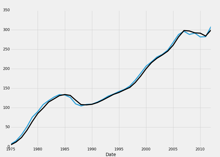
HPI_data.dropna(inplace=True)
print(HPI_data[['TX','TX1yr']])
                    TX       TX1yr
Date
1975-12-31    6.336776    4.559105
1976-12-31   15.000798   11.954152
1977-12-31   30.434104   23.518179
1978-12-31   51.029953   41.978042
1979-12-31   75.975953   64.700665
1980-12-31   89.979964   85.147662
1981-12-31  108.121926   99.016599
1982-12-31  118.210559  114.589927
1983-12-31  127.233791  122.676432
1984-12-31  133.599958  131.033359
1985-12-31  132.576673  133.847016
1986-12-31  126.581048  131.627647
1987-12-31  109.829893  119.373827
1988-12-31  104.602726  107.930502
1989-12-31  108.485926  107.311348
1990-12-31  109.082279  108.727174
1991-12-31  114.471725  113.142303
1992-12-31  121.427564  119.650162
1993-12-31  129.817931  127.009907
1994-12-31  135.119413  134.279735
1995-12-31  141.774551  139.197583
1996-12-31  146.991204  145.786792
1997-12-31  155.855049  152.109010
1998-12-31  170.625043  164.595301
1999-12-31  188.404171  181.149544
2000-12-31  206.579848  199.952853
2001-12-31  217.747701  215.692648
2002-12-31  230.161877  226.962219
2003-12-31  236.946005  235.459053
2004-12-31  248.031552  245.225988
2005-12-31  267.728910  260.589093
2006-12-31  288.009470  281.876293
2007-12-31  296.154296  298.094138
2008-12-31  288.081223  296.999508
2009-12-31  291.665787  292.160280
2010-12-31  281.678911  291.357967
2011-12-31  282.384836  284.001507
2012-12-31  308.404771  299.649905
No more rows with missing data!
Now, we can graph it:
fig = plt.figure()
ax1 = plt.subplot2grid((1,1), (0,0))

HPI_data = pd.read_pickle('fiddy_states3.pickle')
HPI_data['TX1yr'] = HPI_data['TX'].resample('A')
HPI_data.dropna(inplace=True)
print(HPI_data[['TX','TX1yr']])

HPI_data['TX'].plot(ax=ax1)
HPI_data['TX1yr'].plot(color='k',ax=ax1)

plt.legend().remove()
plt.show()
Okay, great. Now just for tutorial purposes, how might we write code that only deletes rows if the full row is NaN?
HPI_data.dropna(how='all',inplace=True)
For the "how" parameter, you can choose between all or any. All requires all data in the row to be NaN for you to delete it. You can also choose "any" and then set a threshold. This threshold will require that many non-NA values to accept the row. See the Pandas documentation for dropna for more information.
Alright, so that's dropna, next we have filling it. With filling, we have two major options again, which is whether to fill forward, backwards. The other option is to just replace the data, but we called that a separate choice. It just so happens that the same function is used to do it, fillna().
Modifying our original code block, with the main change of:
HPI_data.fillna(method='ffill',inplace=True)
Giving us:
fig = plt.figure()
ax1 = plt.subplot2grid((1,1), (0,0))
HPI_data = pd.read_pickle('fiddy_states3.pickle')
HPI_data['TX1yr'] = HPI_data['TX'].resample('A')
HPI_data.fillna(method='ffill',inplace=True)
HPI_data.dropna(inplace=True)
print(HPI_data[['TX','TX1yr']])
HPI_data['TX'].plot(ax=ax1)
HPI_data['TX1yr'].plot(color='k',ax=ax1)
plt.legend().remove()
plt.show()
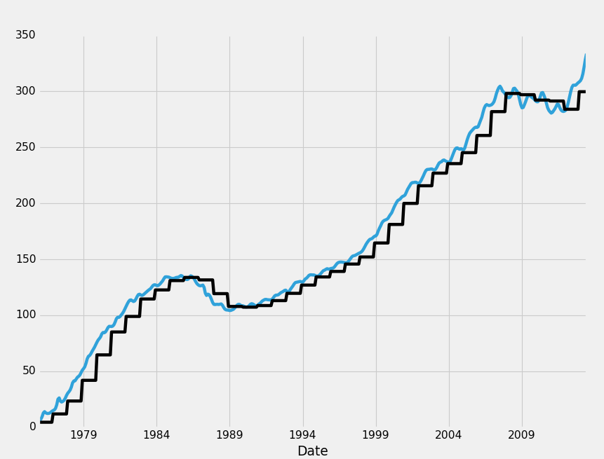
What ffill, or "forward fill" does for is is fills data forward into missing data. Think of it like a sweeping motion where you take data from earlier, sweeping it forward to the missing data. Any case of missing data will be filled witht he most recent non-missing data. Bfill, or backfilling is the opposite:
HPI_data.fillna(method='bfill',inplace=True)
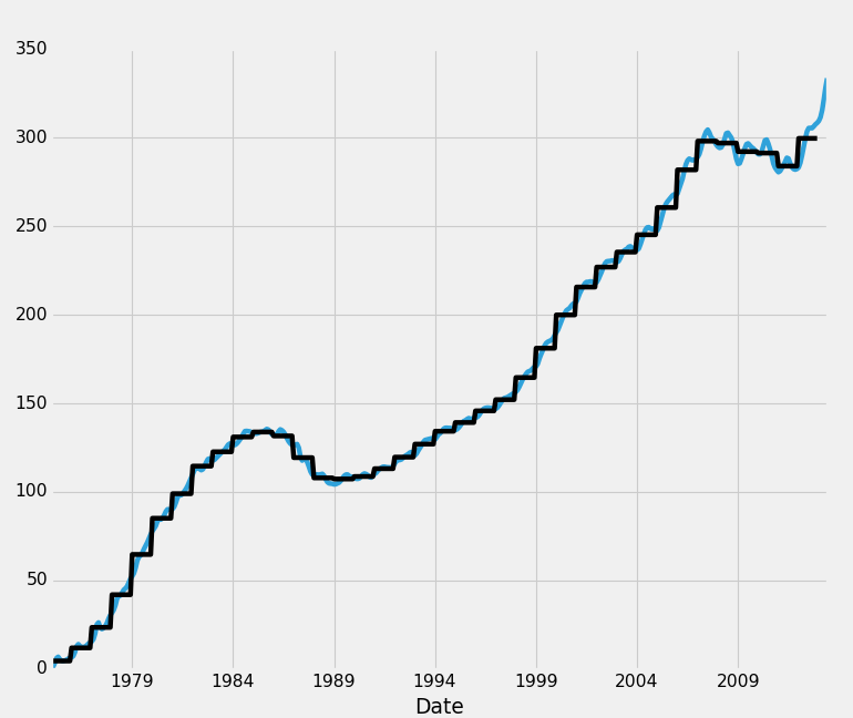
This takes data from the future, and sweeps it backwards to fill in holes.
Now, for the last method, replacing the data. NaN data is relatively worthless data, but it can taint the rest of our data. Take, for example, machine learning, where each row is a feature set and each column is a feature. Data has a very high value to us, and if we have a large amount of NaN data, forfeiting all of the data is a huge bummer. For this reason, you may actually use a replace instead. With most machine learning classifiers, extreme outliers are often ignored in the end as their own data point. Because of this, what many people will do is take any NaN data, and replace it with a value of, say, -99999. This is because, after pre-processing the data, you generally want to convert all features to a range of -1 to positive 1. A data point that is -99999 is a clear and obvious outlier to almost any classifier. NaN data, however, simply cannot be handled at all! Thus, we can replace data, by doing something like the following:
HPI_data.fillna(value=-99999,inplace=True)
Now, in our case, this is an absolutely useless move, but it does have its place in certain forms of data analysis.
Now that we've covered the basics of handling missing data, we're ready to move on. In the next tutorial, we'll talk about another method for smoothing out data that will let us retain our monthly data: Rolling statistics. This will be useful for smoothing out our data as well as gathering some basic statistics on it.
There exists 2 quiz/question(s) for this tutorial. for access to these, video downloads, and no ads.
-
Data Analysis with Python and Pandas Tutorial Introduction
-
Pandas Basics - p.2 Data Analysis with Python and Pandas Tutorial
-
IO Basics - p.3 Data Analysis with Python and Pandas Tutorial
-
Building dataset - p.4 Data Analysis with Python and Pandas Tutorial
-
Concatenating and Appending dataframes - p.5 Data Analysis with Python and Pandas Tutorial
-
Joining and Merging Dataframes - p.6 Data Analysis with Python and Pandas Tutorial
-
Pickling - p.7 Data Analysis with Python and Pandas Tutorial
-
Percent Change and Correlation Tables - p.8 Data Analysis with Python and Pandas Tutorial
-
Resampling - p.9 Data Analysis with Python and Pandas Tutorial
-
Handling Missing Data - p.10 Data Analysis with Python and Pandas Tutorial
-
Rolling statistics - p.11 Data Analysis with Python and Pandas Tutorial
-
Applying Comparison Operators to DataFrame - p.12 Data Analysis with Python and Pandas Tutorial
-
Joining 30 year mortgage rate - p.13 Data Analysis with Python and Pandas Tutorial
-
Adding other economic indicators - p.14 Data Analysis with Python and Pandas Tutorial
-
Rolling Apply and Mapping Functions - p.15 Data Analysis with Python and Pandas Tutorial
-
Scikit Learn Incorporation - p.16 Data Analysis with Python and Pandas Tutorial
