Q-Learning Analysis - Reinforcement Learning w/ Python Tutorial p.3
Welcome to part 3 of the Reinforcement Learning series as well as part 3 of the Q learning parts. Up to this point, we've successfully made a Q-learning algorithm that navigates the OpenAI MountainCar environment. The issue now is, we have a lot of parameters here that we might want to tune. Being able to beat the game is one thing, but we might want to beat it quicker, and maybe even try to explore ways to learn faster. In order to do this, we need to start shedding some light onto what exactly we're doing.
To start, we can track some very basic metrics from within our program. Our starting script:
# objective is to get the cart to the flag.
# for now, let's just move randomly:

import gym
import numpy as np

env = gym.make("MountainCar-v0")

LEARNING_RATE = 0.1

DISCOUNT = 0.95
EPISODES = 25000
SHOW_EVERY = 3000

DISCRETE_OS_SIZE = [20] * len(env.observation_space.high)
discrete_os_win_size = (env.observation_space.high - env.observation_space.low)/DISCRETE_OS_SIZE

# Exploration settings
epsilon = 1  # not a constant, qoing to be decayed
START_EPSILON_DECAYING = 1
END_EPSILON_DECAYING = EPISODES//2
epsilon_decay_value = epsilon/(END_EPSILON_DECAYING - START_EPSILON_DECAYING)


q_table = np.random.uniform(low=-2, high=0, size=(DISCRETE_OS_SIZE + [env.action_space.n]))


def get_discrete_state(state):
    discrete_state = (state - env.observation_space.low)/discrete_os_win_size
    return tuple(discrete_state.astype(np.int))  # we use this tuple to look up the 3 Q values for the available actions in the q-table


for episode in range(EPISODES):
    discrete_state = get_discrete_state(env.reset())
    done = False

    if episode % SHOW_EVERY == 0:
        render = True
        print(episode)
    else:
        render = False

    while not done:

        if np.random.random() > epsilon:
            # Get action from Q table
            action = np.argmax(q_table[discrete_state])
        else:
            # Get random action
            action = np.random.randint(0, env.action_space.n)


        new_state, reward, done, _ = env.step(action)

        new_discrete_state = get_discrete_state(new_state)

        if episode % SHOW_EVERY == 0:
            env.render()
        #new_q = (1 - LEARNING_RATE) * current_q + LEARNING_RATE * (reward + DISCOUNT * max_future_q)

        # If simulation did not end yet after last step - update Q table
        if not done:

            # Maximum possible Q value in next step (for new state)
            max_future_q = np.max(q_table[new_discrete_state])

            # Current Q value (for current state and performed action)
            current_q = q_table[discrete_state + (action,)]

            # And here's our equation for a new Q value for current state and action
            new_q = (1 - LEARNING_RATE) * current_q + LEARNING_RATE * (reward + DISCOUNT * max_future_q)

            # Update Q table with new Q value
            q_table[discrete_state + (action,)] = new_q


        # Simulation ended (for any reson) - if goal position is achived - update Q value with reward directly
        elif new_state[0] >= env.goal_position:
            #q_table[discrete_state + (action,)] = reward
            q_table[discrete_state + (action,)] = 0

        discrete_state = new_discrete_state

    # Decaying is being done every episode if episode number is within decaying range
    if END_EPSILON_DECAYING >= episode >= START_EPSILON_DECAYING:
        epsilon -= epsilon_decay_value


env.close()
For the sake of tinkering, let's first change EPISODES to 4000, just to keep things quicker to iterate for now. Then we'll add a new parameter called STATS_EVERY, and set that to 100.
Next, at the top with our other definitions, let's add
# For stats
ep_rewards = []
aggr_ep_rewards = {'ep': [], 'avg': [], 'max': [], 'min': []}
We will use these to track various values through training to graph them.
Then, let's add episode_reward = 0 to our episode iteration:
for episode in range(EPISODES):
    episode_reward = 0
    ...
Next, after we've received our reward info, we can store it:
        new_state, reward, done, _ = env.step(action)  # was already in our code

        episode_reward += reward
Then at the end of our episodes for loop, we can add:
    ep_rewards.append(episode_reward)
    if not episode % STATS_EVERY:
        average_reward = sum(ep_rewards[-STATS_EVERY:])/STATS_EVERY
        aggr_ep_rewards['ep'].append(episode)
        aggr_ep_rewards['avg'].append(average_reward)
        aggr_ep_rewards['max'].append(max(ep_rewards[-STATS_EVERY:]))
        aggr_ep_rewards['min'].append(min(ep_rewards[-STATS_EVERY:]))
        print(f'Episode: {episode:>5d}, average reward: {average_reward:>4.1f}, current epsilon: {epsilon:>1.2f}')


env.close()  # this was already here, no need to add it again. Just here so you know where we are :)
Finally, at the very end of our script, we can visualize:
plt.plot(aggr_ep_rewards['ep'], aggr_ep_rewards['avg'], label="average rewards")
plt.plot(aggr_ep_rewards['ep'], aggr_ep_rewards['max'], label="max rewards")
plt.plot(aggr_ep_rewards['ep'], aggr_ep_rewards['min'], label="min rewards")
plt.legend(loc=4)
plt.show()
Don't forget to import matplotlib.pyplot as plt at the top.
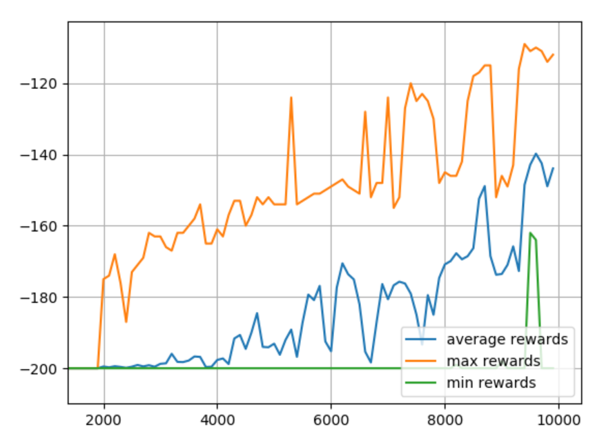
Now we can see the results:
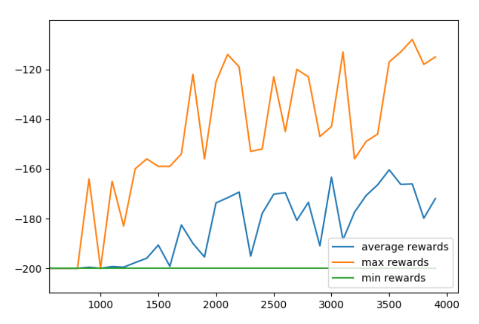
Then, we can tweak certain to things to see if it helps or hurts us. For example, we could try to change our Epsilon decay policy. Let's set that to decay to the very end: END_EPSILON_DECAYING = EPISODES
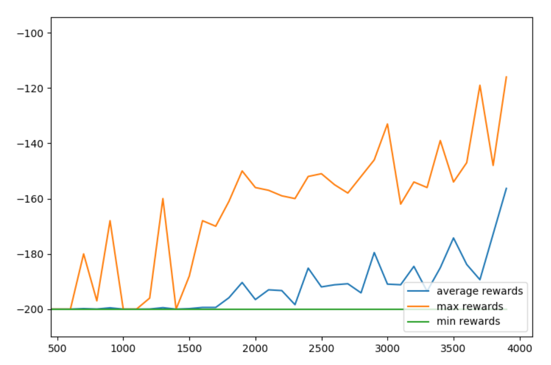
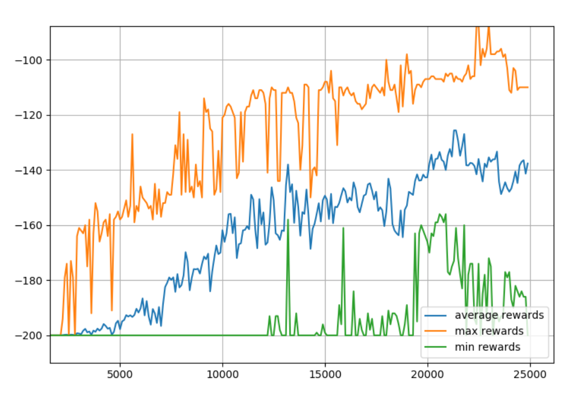
Looks like the 2nd model wanted to keep going, let's raise the episodes to 10,000 and then add plt.grid(True) just before the plt.show()
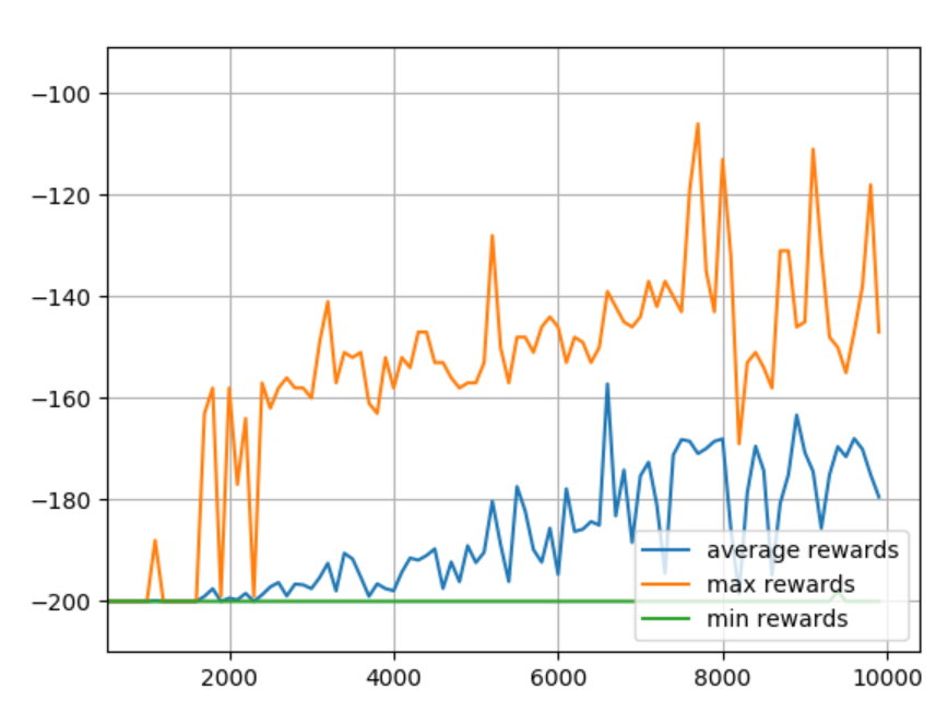
Back to END_EPSILON_DECAYING = EPISODES//2
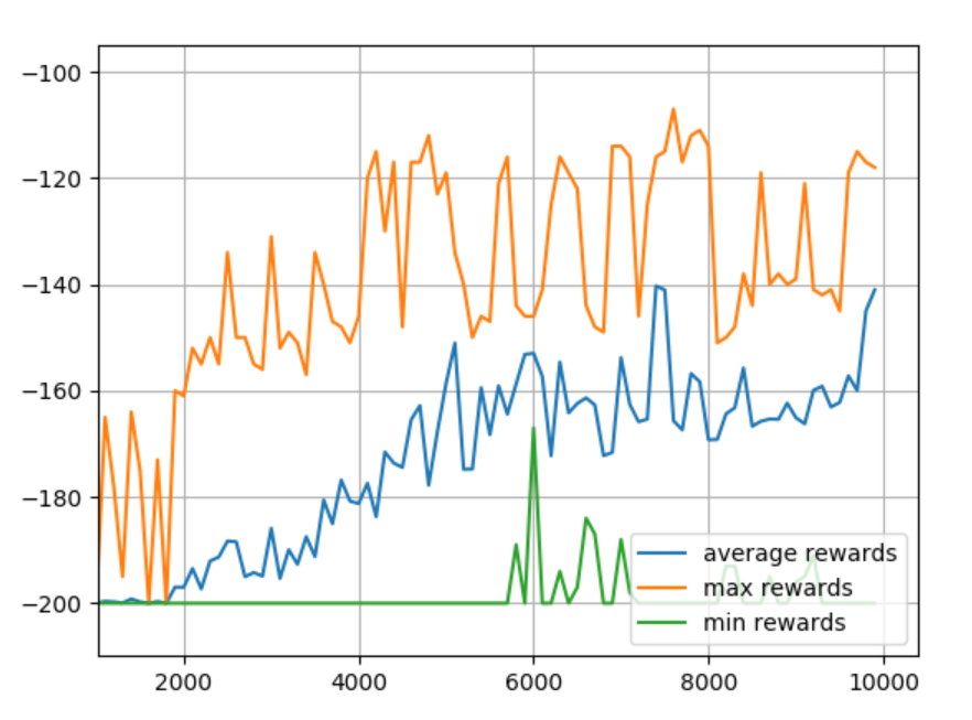
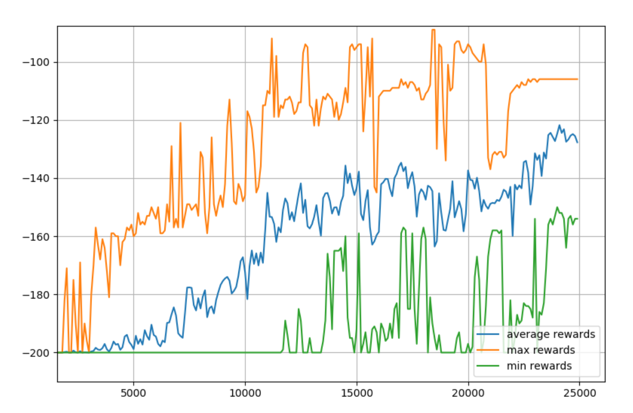
Okay, that seems to be ideal. What about adjusting the observation space? Let's try 40 buckets.
DISCRETE_OS_SIZE = [40] * len(env.observation_space.high)
Looks like it wants more training. Makes sense, because we significantly increased the table size. Let's do 25K episodes.
Seeing this, it looks like we'd like to maybe have the model around 20K episodes since it had high overall rewards, but also the minimum was still high too. Also, we probably want to train models to... I dunno... use them?! So we want to save the final table for sure, but, I propose we save them all! Why?
So we can draw pretty pictures, duh!
...as well as use a model from any point in training.
To start, let's create a new dir called qtables. In here, we're going to save each episode's q-table.
Then, we can throw in a np.save() at the end of the episode loop:
for episode in range(EPISODES):
    ...
    # AT THE END
    np.save(f"qtables/{episode}-qtable.npy", q_table)

env.close()
So this is every single q table. That's a lot of Q tables... so the directory will be ~ 1gb at our discrete observation size. If you want to curtail the size down to more like 100mb, you could do something like
    if episode % 10 == 0:
        np.save(f"qtables/{episode}-qtable.npy", q_table)
Go for 100 if you want more like 10mb of space...etc. Regardless, now we have *all* the q-tables. Turns out our final q-table looks fine:
So we could just use it. So now, rather that initializing a random qtable, you could just np.load that file. Then, you could either continue to update q values, or just use this table to lookup values.
FINALLY! I we didnt save all these Q tables for nothing. Pretty pictures (and video) time!
For this, we'll open a new script.
from mpl_toolkits.mplot3d import axes3d
import matplotlib.pyplot as plt
from matplotlib import style
import numpy as np
style.use('ggplot')
def get_q_color(value, vals):
if value == max(vals):
return "green", 1.0
else:
return "red", 0.3
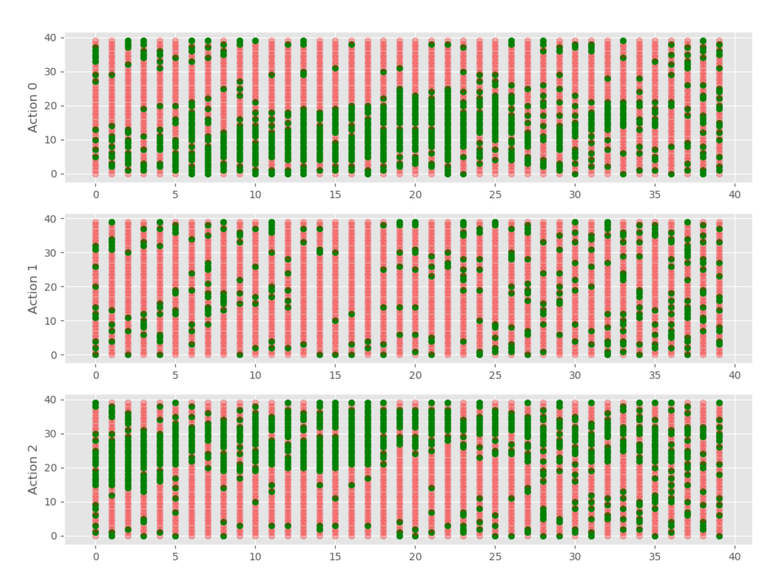
fig = plt.figure(figsize=(12, 9))
ax1 = fig.add_subplot(311)
ax2 = fig.add_subplot(312)
ax3 = fig.add_subplot(313)
i = 24999
q_table = np.load(f"qtables/{i}-qtable.npy")
for x, x_vals in enumerate(q_table):
for y, y_vals in enumerate(x_vals):
ax1.scatter(x, y, c=get_q_color(y_vals[0], y_vals)[0], marker="o", alpha=get_q_color(y_vals[0], y_vals)[1])
ax2.scatter(x, y, c=get_q_color(y_vals[1], y_vals)[0], marker="o", alpha=get_q_color(y_vals[1], y_vals)[1])
ax3.scatter(x, y, c=get_q_color(y_vals[2], y_vals)[0], marker="o", alpha=get_q_color(y_vals[2], y_vals)[1])
ax1.set_ylabel("Action 0")
ax2.set_ylabel("Action 1")
ax3.set_ylabel("Action 2")
plt.show()
So this will graph for us our Q Table for each action, giving us:
Now, we can graph all, or a lot of the episodes. I propose that graphing them all could be a lot. That'd be 25K frames, which would be 7 minutes of video at 60fps. Probably pointless. If we graphed every 10 frames, then that'd be 41 seconds. With this, we can see the Q values changing over time and how the model "learns."
For example, if we set i = 1
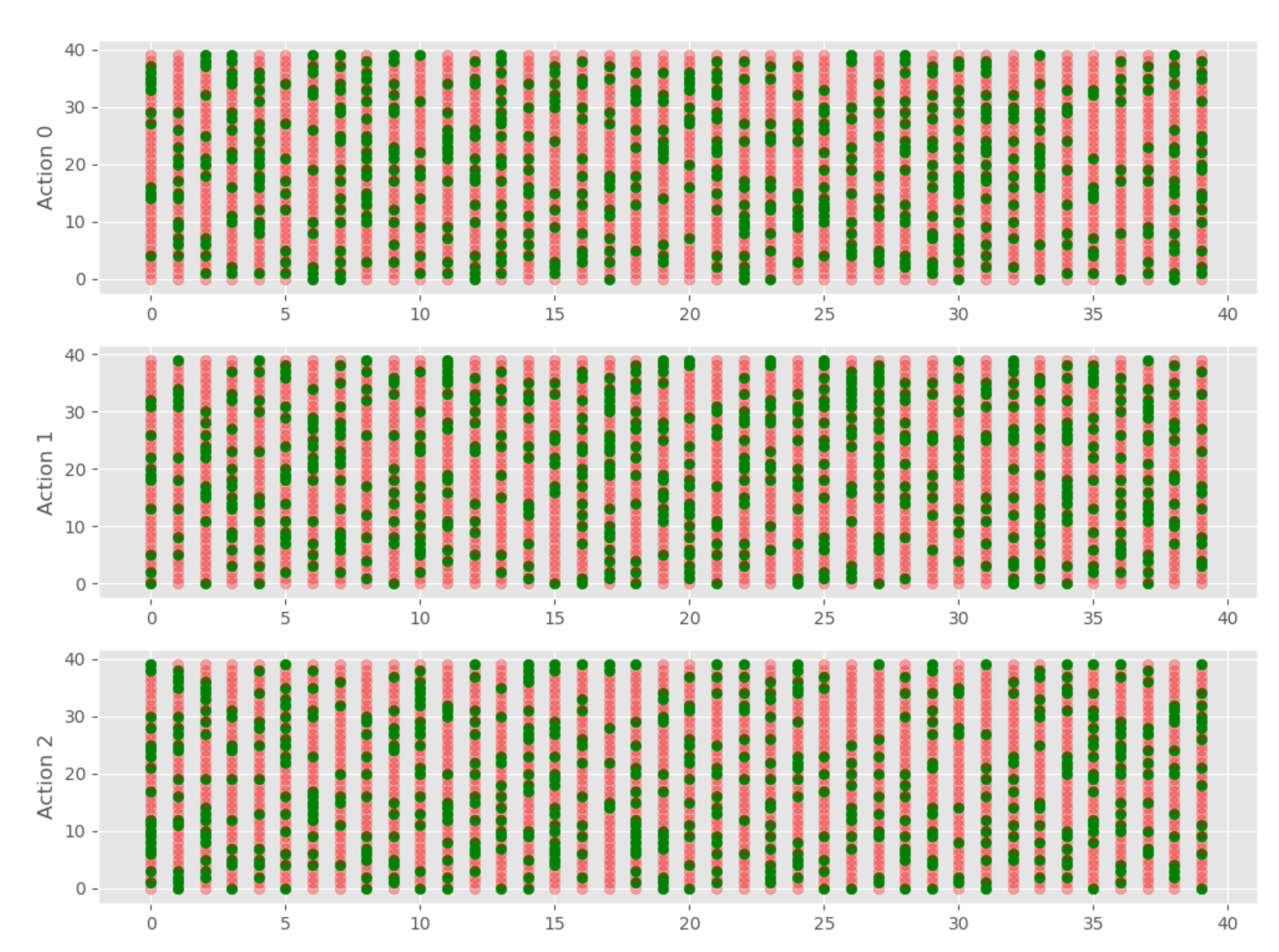
You can clearly see it's random. Not a shocker, we initialized randomly!
Now let's iterate over every 10 q tables, create, and save the chart.
Code is now:
from mpl_toolkits.mplot3d import axes3d
import matplotlib.pyplot as plt
from matplotlib import style
import numpy as np

style.use('ggplot')


def get_q_color(value, vals):
    if value == max(vals):
        return "green", 1.0
    else:
        return "red", 0.3


fig = plt.figure(figsize=(12, 9))


for i in range(0, 25000, 10):
    print(i)
    ax1 = fig.add_subplot(311)
    ax2 = fig.add_subplot(312)
    ax3 = fig.add_subplot(313)

    q_table = np.load(f"qtables/{i}-qtable.npy")

    for x, x_vals in enumerate(q_table):
        for y, y_vals in enumerate(x_vals):
            ax1.scatter(x, y, c=get_q_color(y_vals[0], y_vals)[0], marker="o", alpha=get_q_color(y_vals[0], y_vals)[1])
            ax2.scatter(x, y, c=get_q_color(y_vals[1], y_vals)[0], marker="o", alpha=get_q_color(y_vals[1], y_vals)[1])
            ax3.scatter(x, y, c=get_q_color(y_vals[2], y_vals)[0], marker="o", alpha=get_q_color(y_vals[2], y_vals)[1])

            ax1.set_ylabel("Action 0")
            ax2.set_ylabel("Action 1")
            ax3.set_ylabel("Action 2")

    #plt.show()
    plt.savefig(f"qtable_charts/{i}.png")
    plt.clf()
This will make all of our images, and now we can make videos from them, with:
import cv2
import os


def make_video():
    # windows:
    fourcc = cv2.VideoWriter_fourcc(*'XVID')
    # Linux:
    #fourcc = cv2.VideoWriter_fourcc('M','J','P','G')
    out = cv2.VideoWriter('qlearn.avi', fourcc, 60.0, (1200, 900))

    for i in range(0, 14000, 10):
        img_path = f"qtable_charts/{i}.png"
        print(img_path)
        frame = cv2.imread(img_path)
        out.write(frame)

    out.release()


make_video()
Example video:
In the next tutorial, we're going to create our very own environment to use Q-Learning in.
-
Q-Learning introduction and Q Table - Reinforcement Learning w/ Python Tutorial p.1
-
Q Algorithm and Agent (Q-Learning) - Reinforcement Learning w/ Python Tutorial p.2
-
Q-Learning Analysis - Reinforcement Learning w/ Python Tutorial p.3
-
Q-Learning In Our Own Custom Environment - Reinforcement Learning w/ Python Tutorial p.4
-
Deep Q Learning and Deep Q Networks (DQN) Intro and Agent - Reinforcement Learning w/ Python Tutorial p.5
-
Training Deep Q Learning and Deep Q Networks (DQN) Intro and Agent - Reinforcement Learning w/ Python Tutorial p.6
