Qubits and Gates - Quantum Computer Programming
Hello and welcome to part 2 of the Quantum computer programming tutorials. In this tutorial, I want to talk a bit more about qubits, and subsequently their gates. If you can believe it, I only told you part of the story!
Before this, I want to take a moment to address some of the most common questions that I got from part 1.
Possible states vs considering states
There still seemed to be some confusion about the difference between a classical computer's ability to analyze states and a quantum computer. The thing I heard most was that classical bits can store 2^nbits of information. This is *of course* true. Given `n` bits, there are `2^n_bits` combinations possible. But, can a classical computer actually consider `2^n_bits` of possibilities at once? In true parallel? No. This is what a quantum computer *can* do. Given a single pass through a classical circuit, you can only consider `2*n_bits`. A quantum computer, on a single pass through a quantum circuit, can consider up to `2^n_bits` *logically*, all at once, in parallel. This is the quantum difference. That is what you're going to struggle with mentally to make sense of.How is this useful? How can I make money with this? Will I get a job?
Ask not what quantum computing can do for you, ask what you can do for quantum computing. If you want to just make money as a programmer, this is not yet the field for you, come back in a few decades. You should be looking into web development, machine learning or data analysis, which I also cover. What do we do with it though? These are the same questions people asked from the 50's to the 70s and 80s about classical computers. A small handful of people realized what they could do in the computer industry for profit, and these were pioneers and visionaries that generated billions for themselves and trillions for the world. An even larger number of the early players with classical computers were there purely out of passion and interest in the technology, without any thought about the possibility of profit other than maybe to get their hands on more hardware. It was just interesting and fun to them. Quantum Computing right now is for the curious and passionate, or for the visionary pioneer who plans to change the world. The people interested in being at the forefront of a new age. You're not going to get a job with quantum computing today from watching some unqualified youtuber talk about quantum computing. You're going to have to wait a while for some employer to pay you some cash to tell you what to do with quantum computing. There's nothing inherently wrong by wanting to seek out an immediately employable skillset, but this is not likely one. Eventually, there will be many optimization and search types of tasks that companies will need someone familiar with this technology to formulate into a program to solve their problems. Like the aforementioned route planning for delivery trucks. Another common one is for Ammonia production. Our current method for Amonia production involves heating things up to about 600* F/ 315* C. Given Amonia's use in fertilizer, this process is a common one, accounting for ~5% of the world's energy use. There's no fundamental reason why this is what we must do to produce Amonia, it's just the only way we know *how*. There are many other molecular interactions like this that both exist today and will in the future. Thus, to answer "what we do with this technology?" ...we aim to answer that question. That's what we do.Back to our Qubit story...
To tell the rest of the story, we will visualize the qubit as a vector in space. The notion that a qubit is a 0, 1, or both is not quite true. The measured qubit will collapse to a 0 or 1 value, yes, and if a qubit starts out with no operations, sure, it's a 0. Then if we apply a not gate, it's going be a 1...but this still isn't the full story of what's happening, or, more importantly, what can happen.
We will use the Bloch sphere to visualize this.
Bloch Sphere
We use the Bloch sphere to represent our Hilbert Space.
A Hilbert space is the extension of a Euclidean space, just for infinite dimensions.
Our qubit is represented by a vector in this space. This vector doesn't necessarily map to a 0 or 1 value
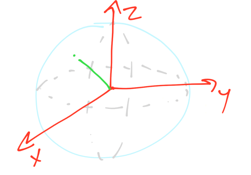
For example, here's our bloch sphere:
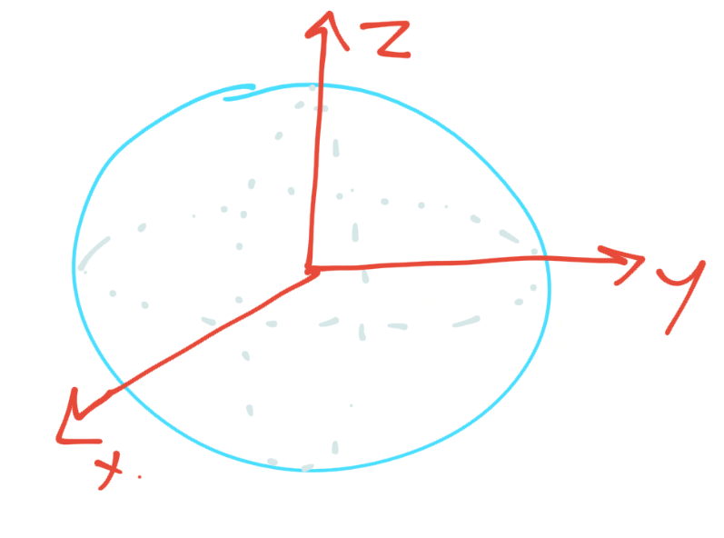
Very pretty, I know. This sphere, at the top and bottom, have values that we can map to classical 0 or 1:
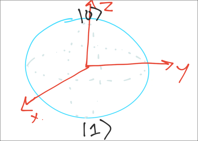
At the "top" of the sphere, we have a zero, this is just the notation for the qubit as a zero |0>
The bottom is a 1 |1>
So then our Qubit is a vector in this space. Pretend for me my green line is straight.
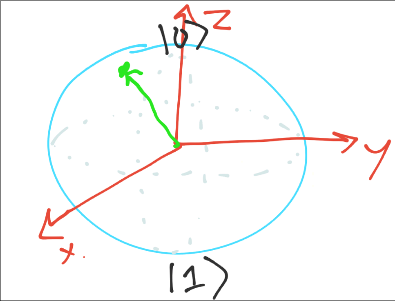
If we took a measurement, this vector here would collapse to a 0 or a 1. On average, this is going to collapse towards the 0 more often.
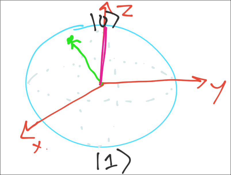
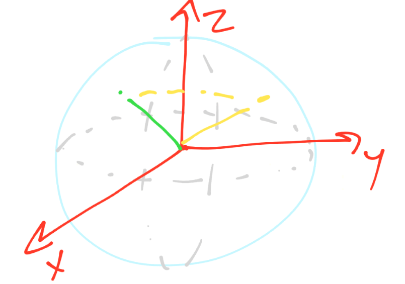
The purple line denotes the collapsed vector value after a measurement has been taken. Do note, however, this vector was not perfectly aligned up to the 0. Sometimes, this qubit will be a 1.
If that wasn't enough to deal with, there are more gate operations than just a not (thought even these in succession can do interesting things). If you were to apply a not here, take note what you think would happen.
Next, there are gates that also do other things, like rotating a vector. For example, you might have a gate that takes the following vector:
and transforms it to:
Now this might currently collapse with the same probabilities, but there are other gates that might rotate in other ways, other gates that will depend on factors like this.
The best way we can get a feel for this is by tinkering with it, however, so let's tinker...because, to be honest, my drawing skills are not the greatest!
To begin, I am going to make a bunch of imports for things we plan to use:
import qiskit as q
from qiskit.tools.visualization import plot_bloch_multivector
from qiskit.visualization import plot_histogram
from matplotlib import style
#style.use("dark_background") # I am using dark mode notebook, so I use this to see the chart.
# to use dark mode:
# edited '/usr/local/lib/python3.7/dist-packages/qiskit/visualization/bloch.py line 177 self.font_color = 'white'
# edited '/usr/local/lib/python3.7/dist-packages/qiskit/visualization/counts_visualization.py line 206     ax.set_facecolor('#000000')
%matplotlib inline


statevec_simulator = q.Aer.get_backend("statevector_simulator")
qasm_sim = q.Aer.get_backend('qasm_simulator')

def do_job(circuit):
    job = q.execute(circuit, backend=statevec_simulator)
    result = job.result()
    statevec = result.get_statevector()

    n_qubits = circuit.n_qubits
    circuit.measure([i for i in range(n_qubits)], [i for i in range(n_qubits)])

    qasm_job = q.execute(circuit, backend=qasm_sim, shots=1024).result()
    counts = qasm_job.get_counts()

    return statevec, counts
Okay so now we've got our simulator setup and then we have a function that will run our job for us and return the state vector and the counts for us, since we're going to be doing this a lot. Now we just make a circuit and run it.
Let's start with something super basic:
circuit = q.QuantumCircuit(2,2)  # 2 qubits, 2 classical bits
statevec, counts = do_job(circuit)
Just an initialized circuit, does nothing. Both qubits should just be 0s always, but let's get a visual:
plot_bloch_multivector(statevec)

So now you can see the vectors! First off, what does adding a Hadamard gate do to the vector? We know this gate puts the qubit in superposition, but what will it look like on the Bloch sphere?
circuit = q.QuantumCircuit(2,2)  # 2 qubits, 2 classical bits
circuit.h(0)  # hadamard gate on qubit0
statevec, counts = do_job(circuit)
plot_bloch_multivector(statevec)

Now, what if we entangle qubit 0 and 1 here, with a cnot gate? What will that look like?
circuit = q.QuantumCircuit(2,2)  # 2 qubits, 2 classical bits
circuit.h(0)  # hadamard gate on qubit0
circuit.cx(0,1)  # controlled not control: 0 target: 1
statevec, counts = do_job(circuit)
plot_bloch_multivector(statevec)

Notice how this cnot entanglement, despite having a target on qubit 1, has actually changed qubit 0's vector. From tutorial 1, you might have instead had the impression that a controlled-not gate just impacted the target qubit.
What will the distribution of measurements be here?
plot_histogram([counts], legend=['output'])

No surprise here, I don't think.
What happens if we have 3 qubits, where qubit at index 2 is controlled by qubit 0 and 1, both of which are in superposition? Try to imagine what the Bloch spheres will look like as well as our distribution?
Could we just do:
circuit = q.QuantumCircuit(3,3)  # 2 qubits, 2 classical bits
circuit.h(0)
circuit.h(1)
circuit.cx(0,2)
circuit.cx(1,2)
circuit.draw()
It would appear that no, we cannot do this, at least it would not be what we expect. Just to show quickly:
statevec, counts = do_job(circuit)
plot_bloch_multivector(statevec)

plot_histogram([counts], legend=['output'])

Luckily, there is actually a way to do this the way we intended, the ccx gate. This is the controlled controlled not gate! It works like what we intended where the target qubit just has 2 control bits, rather than 1.
Imagine having 2 control qubits, both of which are in superposition and nothing more. What's this mean for your target qubit? At what probability will this qubit be a 1?
circuit = q.QuantumCircuit(3,3)  # 3 qubits, 3 classical bits
circuit.h(0)
circuit.h(1)
circuit.ccx(0,1,2)
circuit.draw()
statevec, counts = do_job(circuit)
plot_bloch_multivector(statevec)

One last chance to amend your guesses!
plot_histogram([counts], legend=['output'])

So this is a rather interesting distribution, and we could spend some time pondering on it for sure. I am mostly interested in qubit at index 2 though.
Do we always need to have the same size register for our qubits and bits? What about when we go to measure?
When creating our quantum circuit, we absolutely do not need the same sized registers. We might have 500 qubits, but only care about 1 of those qubits, which we'll map to a classical bit.
When we're mapping bits to bits, however, it obviously does matter that we have a 1 to 1 relationship.
So let's take the exact same circuit gates above, but change the circuit slightly:
circuit = q.QuantumCircuit(3,1) # 3 qubits, only 1 classical bit
So now our circuit will only output 1 classical bit. When we go to measure, we will inform qiskit which qubit will map to this classical bit.
circuit.h(0)  # hadamard
circuit.h(1)  # hadamard
circuit.ccx(0,1,2)  # controlled controlled not
circuit.draw()
circuit.measure([2], [0])  # map qubit @ index 2, to classical bit idx 0.
result = q.execute(circuit, backend=qasm_sim, shots=1024).result()
counts = result.get_counts()
plot_histogram([counts], legend=['output'])

Does that make sense to you? Qubit index 2 has a 23% chance of being a 1?
If you have qubit 0 with a 50/50 split of being 0 or 1, and then qubit 1 also has a 50/50 chance. This seems like a 50% chance of a 50% chance, so 25% chance sounds correct to me.
There are also rotations we can apply to a given axis (x, y, z). These rotations may or may not immediately impact the actual measured values immediately, but combinations of gates like this, superpositions, and entanglements compounding these changes can produce interesting results.
import math

circuit = q.QuantumCircuit(3,3)  # even-sized registers again so we can use our function
circuit.h(0)  # hadamard
circuit.h(1)  # hadamard
circuit.ccx(0,1,2)  # controlled controlled not


statevec, counts = do_job(circuit)
plot_bloch_multivector(statevec)
So we've seen this one before, nothing too fancy. But, it turns out, there's more to quantum life than controlled nots and superpositions.
How about rotations? We can issue a rotation along any given axis we want. Let's play with the x axis first for qubit @ index 2:
circuit = q.QuantumCircuit(3,3)  # even-sized registers again so we can use our function
circuit.h(0)  # hadamard
circuit.h(1)  # hadamard
circuit.ccx(0,1,2)  # controlled controlled not
circuit.rx(math.pi, 2)

statevec, counts = do_job(circuit)
plot_bloch_multivector(statevec)

This arrow is rotating around that x axis. A half rotation is pi. So pi*2 would put us where we started. What about pi/2?
circuit = q.QuantumCircuit(3,3)  # even-sized registers again so we can use our function
circuit.h(0)  # hadamard
circuit.h(1)  # hadamard
circuit.ccx(0,1,2)  # controlled controlled not
circuit.rx(math.pi/2, 2)

statevec, counts = do_job(circuit)
plot_bloch_multivector(statevec)

Oh, that's interesting. Looks like we've found ourself a way to entangle this qubit with 2 others, each in a 50/50 state...and yet... is this also not in a 25% state, but actually in a 50/50 state too? Let's see:
circuit = q.QuantumCircuit(3,3)
circuit.h(0)  # hadamard
circuit.h(1)  # hadamard
circuit.ccx(0,1,2)  # controlled controlled not
circuit.rx(math.pi/2, 2)
circuit.draw()
circuit.measure([2], [0])  # map qubit @ index 2, to classical bit idx 0.
result = q.execute(circuit, backend=qasm_sim, shots=1024).result()
counts = result.get_counts()
plot_histogram([counts], legend=['output'])

It sure is back in the 50/50 state, despite being controlled by a 50% chance * another 50% chance. Very interesting! So we're able to use our circuits to create intersting versions of these relationships. Could it get any more interesting? So far we've been working with making our Qubits whole numbers on specific axis and it's been easy for us to presume what's going to happen.
What about...
circuit = q.QuantumCircuit(3,3)  # even-sized registers again so we can use our function
circuit.h(0)  # hadamard
circuit.h(1)  # hadamard
circuit.ccx(0,1,2)  # controlled controlled not
circuit.rx(math.pi/4, 2)

statevec, counts = do_job(circuit)
plot_bloch_multivector(statevec)

Well now isn't that interesting?
plot_histogram([counts], legend=['output'])

Remember, this is a simulated "perfect" machine. Look at how many possibilities we've got with just 3 qubits? Looks like 2^nbits to me.
...but thats just the X axis my friends. What about the other 2?!
circuit = q.QuantumCircuit(3,3)  # even-sized registers again so we can use our function
circuit.h(0)  # hadamard
circuit.h(1)  # hadamard
circuit.ccx(0,1,2)  # controlled controlled not
circuit.rx(math.pi/4, 2)
circuit.rz(math.pi, 2)
statevec, counts = do_job(circuit)
plot_bloch_multivector(statevec)

plot_histogram([counts], legend=['output'])

circuit = q.QuantumCircuit(3,3)  # even-sized registers again so we can use our function
circuit.h(0)  # hadamard
circuit.h(1)  # hadamard
circuit.ccx(0,1,2)  # controlled controlled not
circuit.rx(math.pi/4, 2)
circuit.rz(math.pi, 2)
circuit.ry(math.pi, 2)
statevec, counts = do_job(circuit)
plot_bloch_multivector(statevec)

plot_histogram([counts], legend=['output'])

Obviously, we don't even need to rotate by such pretty numbers, but I think you get the idea. We can apply gates to do ... well, a lot of things to that vector. Then subsequent qubits can rely upon it. For example:
circuit = q.QuantumCircuit(4,4)  # even-sized registers again so we can use our function
circuit.h(0)  # hadamard
circuit.h(1)  # hadamard
circuit.ccx(0,1,2)  # controlled controlled not
circuit.rx(math.pi/4, 2)
circuit.rz(math.pi, 2)
circuit.ry(math.pi, 2)
circuit.cx(2,3)
statevec, counts = do_job(circuit)
plot_bloch_multivector(statevec)

Finally, why is qubit 2 (index: 2) vector changing when it's a control?
There are many gates, you can find them all here: https://qiskit.org/documentation/api/qiskit.circuit.QuantumCircuit.html in the methods summary, along with all the other methods you can use with your circuit.
For the ultra curious among us, you can also check out https://github.com/Qiskit/qiskit-terra/tree/master/qiskit/extensions/standard for the actual source code for these simulated gates. It's pretty cool if you ask me to see these applied in Python code.
Also, remember that you can use a controlled not gate to first dictate a bits position, or you could apply it after the fact.
circuit = q.QuantumCircuit(4,4)  # even-sized registers again so we can use our function
circuit.h(0)  # hadamard
circuit.h(1)  # hadamard
circuit.rx(math.pi/4, 2)
circuit.rz(math.pi, 2)
circuit.ry(math.pi, 2)
circuit.cx(2,3)

# moving this down here to the very end:
circuit.ccx(0,1,2)  # controlled controlled not
circuit.draw()
statevec, counts = do_job(circuit)
plot_bloch_multivector(statevec)

plot_histogram([counts], legend=['output'])

What happens if we slap a bunch of hadamard gates at the end?
circuit = q.QuantumCircuit(4,4)  # even-sized registers again so we can use our function
circuit.h(0)  # hadamard
circuit.h(1)  # hadamard
circuit.rx(math.pi/4, 2)
circuit.rz(math.pi, 2)
circuit.ry(math.pi, 2)
circuit.cx(2,3)
# moving this down here to the very end:
circuit.ccx(0,1,2)  # controlled controlled not

circuit.h(0)
circuit.h(1)
circuit.h(2)
circuit.h(3)

circuit.draw()
statevec, counts = do_job(circuit)
plot_bloch_multivector(statevec)

plot_histogram([counts], legend=['output'])

Well I was just trying to have some fun. I am actually kind of confused with this one. This one doesn't appear to me like it's going to add up to a 100% distribution. More like 50%.
The ending hadamard gates also appear somewhat jumbled and confusing to me. To correct for this, we can use .barrier() to clean it up. It should be noted that the barrier's function is to force the optimizer (a thing in the backend that you don't have to worry about, but it optimizes your circuits) to not optimize only the chunks, and not the whole circuit. Basically if you have 2 chunks, the optimizer optimizes the two chunks, but not them together. That said, I...think I have only seen people using the barrier() for drawing cosmetic reasons. I am sure that's because I am just getting started here and there's probably a more legitimate use for barrier besides just cosmetics.
circuit = q.QuantumCircuit(4,4)  # even-sized registers again so we can use our function
circuit.h(0)  # hadamard
circuit.h(1)  # hadamard
circuit.rx(math.pi/4, 2)
circuit.rz(math.pi, 2)
circuit.ry(math.pi, 2)
circuit.cx(2,3)
# moving this down here to the very end:
circuit.ccx(0,1,2)  # controlled controlled not
circuit.barrier()
circuit.h(0)
circuit.h(1)
circuit.h(2)
circuit.h(3)

circuit.draw()
statevec, counts = do_job(circuit)
plot_bloch_multivector(statevec)
plot_histogram([counts], legend=['output'])

Now, before I stop the pain and leave you guys, one last thing.
What do you think...is there such a thing as a controlled rotation?
...of course!
circuit = q.QuantumCircuit(3,3)  # even-sized registers again so we can use our function
circuit.h(0)  # hadamard
circuit.h(1)  # hadamard
circuit.rx(math.pi*1.25, 2)
circuit.draw()
statevec, counts = do_job(circuit)
plot_bloch_multivector(statevec)

circuit = q.QuantumCircuit(3,3)  # even-sized registers again so we can use our function
circuit.h(0)  # hadamard
circuit.h(1)  # hadamard
circuit.x(2)
circuit.crz(math.pi, 1, 2)  # theta, control, target
circuit.draw()
statevec, counts = do_job(circuit)
plot_bloch_multivector(statevec)

Finally, what about gates that do not exist in Qiskit?
For example, a CRY (controlled rotation for y axis) doesn't currently exist in Qiskit, but all of these gates can be built.
You can build almost everything with hadamards and controlled not gates. If you want rotations, then you will need those too, but once you have just these basic types, you can do anything.
For example, a controlled rotation on y could look like:
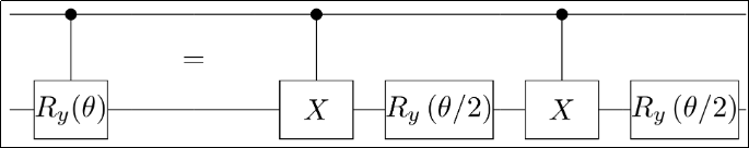
Which is from: https://quantumcomputing.stackexchange.com/questions/6472/implementing-a-complex-circuit-for-a-szegedy-quantum-walk-in-qiskit/6474
There's another example using u3 gates: https://quantumcomputing.stackexchange.com/questions/2143/how-can-a-controlled-ry-be-made-from-cnots-and-rotations/2144#2144
...which I haven't even talked about! But, we've got to stop at some point, and that point is now. In the coming video, I'd like to talk about some of the known quantum algorithms that offer us insights into what quantum computers can do as well as to serve as decent examples of how to actually build a quantum circuit to do a thing.
I encourage you to also consider how you might manipulate a qubit's vector on the bloch sphere. Think of a goal for the vector, then attempt to write a circuit to implement that. For example, try a controled rotation of the Z axis, and see what you can figure out, then maybe try some others.
Til next time!
