Unsupervised Machine Learning: Hierarchical Clustering
Mean Shift cluster analysis example with Python and Scikit-learn
The next step after Flat Clustering is Hierarchical Clustering, which is where we allow the machine to determined the most applicable unumber of clusters according to the provided data.
It is posited that humans are the only species capable of hierarchical thinking to any large degree, and it is only the mammalian brain that exhibits it at all, since some chimps have been able to learn things like sign language.
What actually is hierarchical thinking?
Hierarchical thinking is shown when you can take a structure with many elements, arrange those elements into a pattern, give that pattern a symbol, and then use that symbol as an element in another structure with many elements, repeating this process many times for many layers of "complexity."
One of the easiest examples of hierarchical thinking is written language. First you have lines, then you take those lines and put them together to make shapes, called letters. Next you arrange those letters into patterns and call them words with unique names and meanings for each word. Then we take these words to form patterns of meaning called sentences. Then we put those together to express entire ideas, concepts, and general knowledge.
With this, humans the only species on this planet capable of actually "compounding" their knowledge, building on top of pre-existing knowledge, continually adding layers of complexity, yet easily understanding it because we've employed hierarchical thinking.
This is a fascinating concept to me. For example, consider that:
A little over 300 years ago, we were burning people at the stake and engaging in other torturous acts against them on the grounds that they were witches.
150 years ago, (this tutorial is written in 2015) the United States abolished slavery with the 13th ammendment. While some people still lag behind, we are in general agreement, that all humans are created equal.
Biologically, nothing significant separates us from our cousines of the 1800s and late 1600s. We are the very same people. Consider for a moment how easily you could have been a slave owner, or enslaved (something still occurring today). Or how you could have condemned a witch, or been the witch yourself (something still occurring today).
The only thing separating us now from those times is this degree of hierarchical learning. Time has aided us in our hierarchical learning linearly, though the age of the internet has sped this process of significantly. Looking at the societies still enslaving people, barring those trafficking purely for the money, or the societies who are still burning witches (or similar acts), we can obviously see they are disconnected, quite literally, from the rest of world knowledge.
There are plenty of examples of how knowledge stacks on top of knowledge, and they all point to our "increased" intelligence of today compared to 1,000 years ago as being non-biological.
I've long tried to point out how incredibly basic and simple programming is. You can break down every single program into simple patterns of if statements, while loops, for loops, some functions, maybe some objects if OOP is used, maybe a few other things, but it all breaks down into incredibly basic elements.
There's really nothing complex about programming, nor is there about anything at all. Everything breaks down into simple elements, which are put together into a structure. That structure, again, comprised of simple elements, then becomes an element, still simple, that gets put together into another structure. Humans get it. Dogs don't.
...and, not too surprisingly, computers get it too. Unlike our current knowledge-base mostly leading up to this point, which grew linearly, computers are now allowing us to grow this knowledge-base exponentially.
Now this is just a tiny sliver of hierarchical learning, but it's quite awesome how quickly you can do such a thing.
We're going to employ Python and the Scikit-learn (sklearn) module to do this.
Don't have Python or Sklearn?Python is a programming language, and the language this entire website covers tutorials on. If you need Python, click on the link to python.org and download the latest version of Python.
Scikit-learn (sklearn) is a popular machine learning module for the Python programming language.
The Scikit-learn module depends on Matplotlib, SciPy, and NumPy as well. You can use pip to install all of these, once you have Python.
Don't know what pip is or how to install modules?Pip is probably the easiest way to install packages Once you install Python, you should be able to open your command prompt, like cmd.exe on windows, or bash on linux, and type:
pip install scikit-learn
Having trouble still? No problem, there's a tutorial for that: pip install Python modules tutorial.
If you're still having trouble, feel free to contact us, using the contact in the footer of this website.
There are many methodologies for hierarchical clustering. Since we're using Scikit-learn here, we are using Ward's Method, which works by measuring degrees of minimum variance to create clusters.
The specific algorithm that we're going to use here is Mean Shift.
Let's hop into our example, shall we?
First, let's do the imports:
import numpy as np
from sklearn.cluster import MeanShift
from sklearn.datasets.samples_generator import make_blobs
import matplotlib.pyplot as plt
from matplotlib import style
style.use("ggplot")
NumPy for the swift number crunching, then, from the clustering algorithms of scikit-learn, we import MeanShift.
We're going to be using the sample generator built into sklearn to create a dataset for us here, called make_blobs.
Finally, Matplotlib for the graphing aspects.
centers = [[1,1],[5,5],[3,10]]
X, _ = make_blobs(n_samples = 500, centers = centers, cluster_std = 1)
Above, we're making our example data set. We've decided to make a dataset that originates from three center-points. One at 1,1, another at 5,5 and the other at 3,10. From here, we generate the sample, unpacking to X and y. X is the dataset, and y is the label of each data point according to the sample generation.
This part might confuse some people. We're unpacking to y because we have to, since the make_blobs returns a label, but we do not actually use y, other than to possibly test the accuracy of the algorithm. Remember, unsupervised learning does not actually train against data and labels, it derives structure and labels on its own, it's not derivative.
What we have now is an example data set, with 500 randomized samples around the center points with a standard deviation of 1 for now.
This has nothing to do with machine learning yet, we're just creating a data set. At this point, it would help to visualize the data set, so let's do:
plt.scatter(X[:,0],X[:,1])
plt.show()
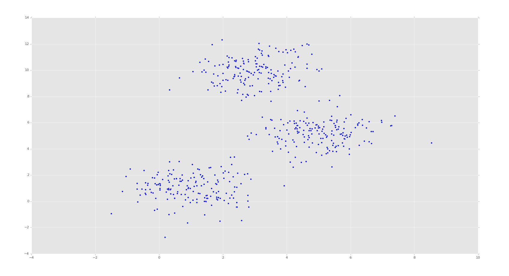
Your example should look similar. Here, we can already identify ourselves the major clusters. There are some points in between the clusters that we might not know exactly where they go, but we can see the clusters.
What we want is the machine to do the same thing. We want the machine to see this data set, without knowing how many clusters there ought to be, and identify the same three clusters we can see are obviously clusters.
For this, we're going to use MeanShift
ms = MeanShift()
ms.fit(X)
labels = ms.labels_
cluster_centers = ms.cluster_centers_
First we initialize MeanShift, then we fit according to the dataset, "X."
Next we populate labels and cluster_centers with the machine-chosen labels and cluster centers. Keep in mind here, the labels are the ones the machine has chosen, these are not the same labels as the unpacked-to "y" variable above.
We could compare the two for an accuracy measurement, but this may or may not be very useful in the end, given the way we're synthetically generating data. If we were to set our standard deviation to, say, 10, there would be signficant overlap. Even if the data originally came from from one cluster, it might actually be a better fit into another. This isn't really a fault of the machine learning algorithm in any way. The data is actually a better fit elsewhere and you were too wild with the standard deviation in the generation.
Instead, it might be a bit better of an accuracy measurement to compare the cluster_centers with the actual cluster centers you started with (centers = [[1,1],[5,5],[3,10]]) to create the random data. We'll see how accurate this is, though it should be a given that: The more samples you have, and the less standard deviation, the more accurate your predicted cluster centers should be compared to the actual ones used to generate the randomized data. If this is not the case, then the machine learning algorithm might be problematic.
We can see the cluster centers and grab the total number of clusters by doing the following:
print(cluster_centers)
n_clusters_ = len(np.unique(labels))
print("Number of estimated clusters:", n_clusters_)
Next, since we're intending to graph the results, we want to have a nice list of colors to choose from:
colors = 10*['r.','g.','b.','c.','k.','y.','m.']
This is just a simple list of red, green, blue, cyan, black, yellow, and magenta multiplied by ten. We should be confident that we're only going to need three colors, but, with hierarchical clustering, we are allowing the machine to choose, we'd like to have plenty of options. This allows for 70 clusters, so that should be good enough.
Now for the plotting code. This code is purely for graphing only, and has nothing to do with machine learning other than helping us petty humans to see what is happening:
for i in range(len(X)):
    plt.plot(X[i][0], X[i][1], colors[labels[i]], markersize = 10)

plt.scatter(cluster_centers[:,0],cluster_centers[:,1],
            marker="x",color='k', s=150, linewidths = 5, zorder=10)

plt.show()
Above, first we're iterating through all of the sample data points, plotting their coordinates, and coloring by their label # as an index value in our color list.
After the for loop, we are calling plt.scatter to scatter plot the cluster centers.
Finally, we show it. You should see something similar to:
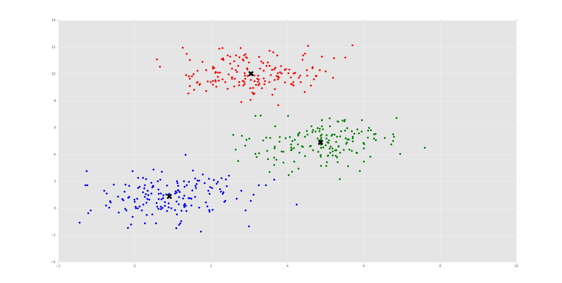
Thus, we can see our machine did it! Very exciting times. We should next peak at the cluster_centers:
[[ 0.86629751  1.03005482]
 [ 4.9038423   5.16998291]
 [ 3.0363859   9.9793174 ]]
Your centers will be slightly different, and the centers will be different every time you run it, since there is a degree of randomness with our sample generation. Regardless, the cluster_centers are darn close to the original values that we created. Very impressive.
From here, try adding more clusters, try increasing the standard deviation. Without getting too absurd, try to give the machine a decent challenge.
Now, let's do a bonus round! How about 3 dimensions? If you want to learn more about 3D plotting, see the 3D plotting with Matplotlib Tutorial.
import numpy as np
from sklearn.cluster import MeanShift# as ms
from sklearn.datasets.samples_generator import make_blobs
import matplotlib.pyplot as plt
from mpl_toolkits.mplot3d import Axes3D
from matplotlib import style
style.use("ggplot")

centers = [[1,1,1],[5,5,5],[3,10,10]]

X, _ = make_blobs(n_samples = 500, centers = centers, cluster_std = 1.5)


ms = MeanShift()
ms.fit(X)
labels = ms.labels_
cluster_centers = ms.cluster_centers_

print(cluster_centers)

n_clusters_ = len(np.unique(labels))

print("Number of estimated clusters:", n_clusters_)

colors = 10*['r','g','b','c','k','y','m']

print(colors)
print(labels)

fig = plt.figure()
ax = fig.add_subplot(111, projection='3d')

for i in range(len(X)):

    ax.scatter(X[i][0], X[i][1], X[i][2], c=colors[labels[i]], marker='o')


ax.scatter(cluster_centers[:,0],cluster_centers[:,1],cluster_centers[:,2],
            marker="x",color='k', s=150, linewidths = 5, zorder=10)

plt.show()
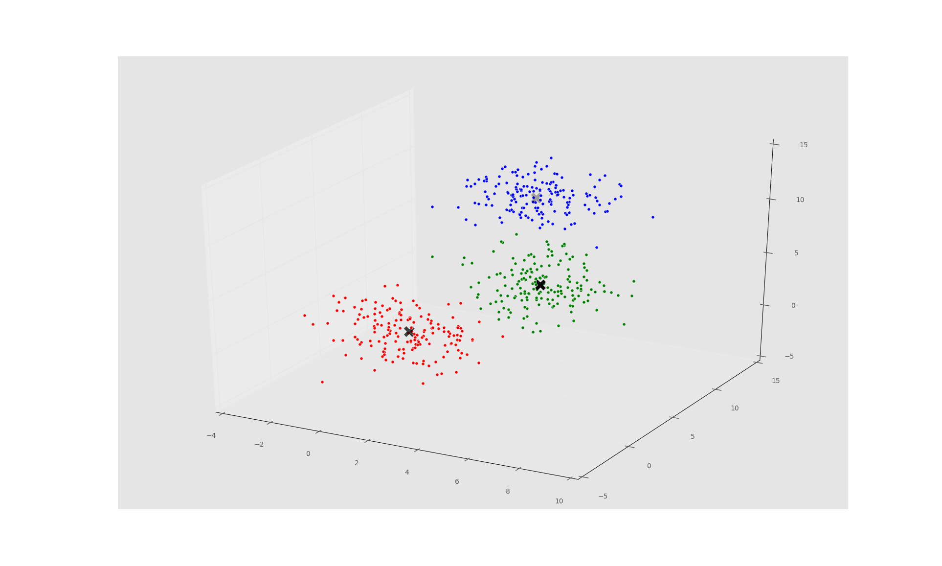
You may regret doing 500 samples on a 3D plot depending on your processing abilities, but feel free to try it. Now the output should be something like:
Machine-Chosen Clusters:
[[ 1.11615056  1.10163911  1.06359602]
 [ 4.84704737  5.19257102  4.83831019]
 [ 2.89080753  9.95938337  9.95381081]]
Actual Centers Used:
[[ 1.0  1.0  1.0]
 [ 5.0  5.0  5.0]
 [ 3.0  10.0 10.0]]
That's quite accurate. Just like before, you might be thinking "well I could have easily figured this one out." Sure, that's true. 2D and 3D is easy. Try 15D, or 15,000D, don't forget to use PCA.
There exists 1 challenge(s) for this tutorial. for access to these, video downloads, and no ads.
There exists 2 quiz/question(s) for this tutorial. for access to these, video downloads, and no ads.
That's all for now on this topic. For other tutorials, head to the
