Applying Comparison Operators to DataFrame - p.12 Data Analysis with Python and Pandas Tutorial

Welcome to part 12 of the Data Analysis with Python and Pandas tutorial series. In this tutorial, we're goign to talk briefly on the handling of erroneous/outlier data. Just because data is an outlier, it does not mean it is erroneous. A lot of times, an outlier data point can nullify a hypothesis, so the urge to just get rid of it can be high, but this isn't what we're talking about here.

What would an erroneous outlier be? An example I like to use is when measuring fluctuations in something like, say, a bridge. As bridges carry weight, they can move a bit. In storms, that can wiggle about a bit, there is some natural movement. As time goes on, and supports weaken, the bridge might move a bit too much, and eventually need to be reinforced. Maybe we have a system in place that constantly measures fluctuations in the bridge's height.

Some distance sensors use lasers, others bounce sound waves. Whichever you want to pretend we're using, it doesn't matter. We'll pretend sound waves. The way these work is they emit sound waves from the trigger, which then bounce of the object in front, coming back to the receiver. From here, amount of time for this entire operation to occur is accounted for. Since the speed of sound is a constant, we can extrapolate from the time this process took, the distance the sound waves traveled. The problem is, this is only a measure of how far the sound waves traveled. There is no 100% certainty that they went to the bridge and back, for example. Maybe a leaf fell just as the measurement was being taken and bounced the signal around a bunch before it got back to the receiver, who knows. Let's say, for example though, you had the following readings for the bridge:

bridge_height = {'meters':[10.26, 10.31, 10.27, 10.22, 10.23, 6212.42, 10.28, 10.25, 10.31]}

We can visualize this:

import pandas as pd
import matplotlib.pyplot as plt
from matplotlib import style

style.use('fivethirtyeight')

bridge_height = {'meters':[10.26, 10.31, 10.27, 10.22, 10.23, 6212.42, 10.28, 10.25, 10.31]}
df = pd.DataFrame(bridge_height)

df.plot()
plt.show()

So, did the bridge just get abducted by aliens? Since we have more normal readings after this, it's more likely that 6212.42 was just a bad reading though. We can tell visually that it is an outlier, but how could we detect this via our program?

We realize this is an outlier because it differs so greatly from the other values, as well as the fact that it suddenly jumps and drops way more than any of the others. Soundes like we're just applying standard deviation here. Let's use that to automatically detect this bad reading.

df['STD'] = pd.rolling_std(df['meters'], 2)
print(df)

Output:

    meters          STD
0    10.26          NaN
1    10.31     0.035355
2    10.27     0.028284
3    10.22     0.035355
4    10.23     0.007071
5  6212.42  4385.610607
6    10.28  4385.575252
7    10.25     0.021213
8    10.31     0.042426

Next, we can grab the standard deviation for the whole set like:

df_std = df.describe()
print(df_std)
df_std = df.describe()['meters']['std']
print(df_std)

Output:

            meters          STD
count     9.000000     8.000000
mean    699.394444  1096.419446
std    2067.384584  2030.121949
min      10.220000     0.007071
25%      10.250000     0.026517
50%      10.270000     0.035355
75%      10.310000  1096.425633
max    6212.420000  4385.610607
2067.38458357

First, we get all the description. Mostly just showing that so you see how we're working with the data. Then, we get get straight to the meters' std, which is 2067 and some change. That's a pretty high figure, but it's still much lower than the STD for that major fluctuation (4385). Now, we can run through and remove all data that has a standard deviation higher than that.

This allows us to learn a new skill: Logically modifying the dataframe! What we can do is something like:

df = df[ (df['STD'] < df_std) ]
print(df)

Output:

   meters       STD
1   10.31  0.035355
2   10.27  0.028284
3   10.22  0.035355
4   10.23  0.007071
7   10.25  0.021213
8   10.31  0.042426

Then we can graph all of this:

import pandas as pd
import matplotlib.pyplot as plt
from matplotlib import style

style.use('fivethirtyeight')

bridge_height = {'meters':[10.26, 10.31, 10.27, 10.22, 10.23, 6212.42, 10.28, 10.25, 10.31]}
df = pd.DataFrame(bridge_height)

df['STD'] = pd.rolling_std(df['meters'], 2)
print(df)

df_std = df.describe()
print(df_std)
df_std = df.describe()['meters']['std']
print(df_std)


df = df[ (df['STD'] < df_std) ]
print(df)

df['meters'].plot()
plt.show()

Output:

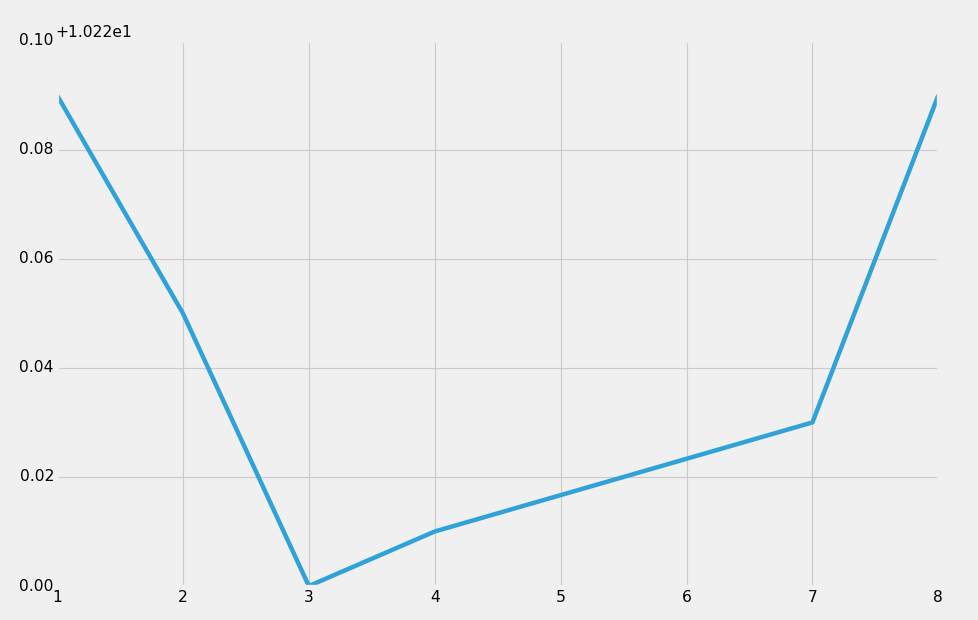
The new line we just learned was this df = df[ (df['STD'] < df_std) ]. How did that work? First, we start by re-defining df. We're saying df is equal now to df, where df['STD'] is less than the overall df_std that we calculated before. Thus, the only remaining data here will be data where the standard deviation is less than that 2067.

Again, we're allowed to just remove this data when we know it's erroneous. Deleting data because it just doesn't "suit" you is almost always a bad idea.

There exists 1 quiz/question(s) for this tutorial. Sign up to +=1 for access to these, video downloads, and no ads.

The next tutorial: Joining 30 year mortgage rate - p.13 Data Analysis with Python and Pandas Tutorial