Percent Change and Correlation Tables - p.8 Data Analysis with Python and Pandas Tutorial

Welcome to Part 8 of our Data Analysis with Python and Pandas tutorial series. In this part, we're going to do some of our first manipulations on the data. Our script up to this point is:

import Quandl
import pandas as pd
import pickle

# Not necessary, I just do this so I do not show my API key.
api_key = open('quandlapikey.txt','r').read()

def state_list():
    fiddy_states = pd.read_html('https://simple.wikipedia.org/wiki/List_of_U.S._states')
    return fiddy_states[0][0][1:]
    

def grab_initial_state_data():
    states = state_list()

    main_df = pd.DataFrame()

    for abbv in states:
        query = "FMAC/HPI_"+str(abbv)
        df = Quandl.get(query, authtoken=api_key)
        print(query)
        if main_df.empty:
            main_df = df
        else:
            main_df = main_df.join(df)
            
    pickle_out = open('fiddy_states.pickle','wb')
    pickle.dump(main_df, pickle_out)
    pickle_out.close()        

HPI_data = pd.read_pickle('fiddy_states.pickle')

Now we can modify columns like so:

HPI_data['TX2'] = HPI_data['TX'] * 2
print(HPI_data[['TX','TX2']].head())

Output:

                   TX        TX2
Date                            
1975-01-31  32.617930  65.235860
1975-02-28  33.039339  66.078677
1975-03-31  33.710029  67.420057
1975-04-30  34.606874  69.213747
1975-05-31  34.864578  69.729155

We could have also not made a new column, just re-defined the original TX if we so chose. Removing the whole "TX2" bit of code from our script, let's visualize what we have right now. At the top of your script:

import matplotlib.pyplot as plt
from matplotlib import style
style.use('fivethirtyeight')

Then at the bottom:

HPI_data.plot()
plt.legend().remove()
plt.show()

Output:

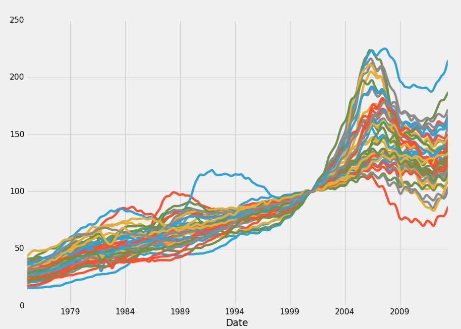
Hmm, interesting, what's going on? All those prices seem to converge perfectly in 2000! Well, this is just when the 100.0% of the index starts. We could get by with this, but I am just simply not a fan. What about some sort of percent change? Turns out, Pandas has you covered here with all sorts of "rolling" statistics. We can slap on a basic one, like this:

def grab_initial_state_data():
    states = state_list()

    main_df = pd.DataFrame()

    for abbv in states:
        query = "FMAC/HPI_"+str(abbv)
        df = Quandl.get(query, authtoken=api_key)
        print(query)
        df = df.pct_change()
        print(df.head())
        if main_df.empty:
            main_df = df
        else:
            main_df = main_df.join(df)
            
    pickle_out = open('fiddy_states2.pickle','wb')
    pickle.dump(main_df, pickle_out)
    pickle_out.close()

grab_initial_state_data() 

Mainly, you are wanting to take note of: df = df.pct_change(), We'll re run this, saving to fiddy_states2.pickle. Notably, we could also attempt to modify the original pickle, rather than re-pulling. That was the point of the pickle, after all. If I didn't have hindsight bias, I might agree with you.

HPI_data = pd.read_pickle('fiddy_states2.pickle')

HPI_data.plot()
plt.legend().remove()
plt.show()

Output:

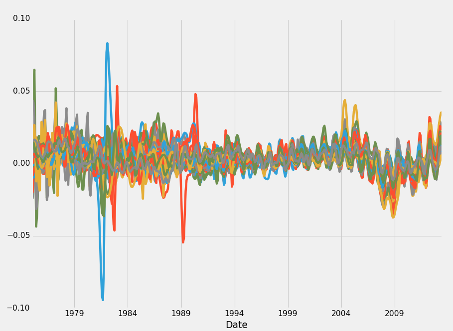
Not quite what I was thinking, unfortunately. I want a traditional % Change chart. This is %change from the last reported value. We could increase it, and do something like a rolling % of the last 10 values, but still not quite what I want. Let's try something else:

def grab_initial_state_data():
    states = state_list()

    main_df = pd.DataFrame()

    for abbv in states:
        query = "FMAC/HPI_"+str(abbv)
        df = Quandl.get(query, authtoken=api_key)
        print(query)
        df[abbv] = (df[abbv]-df[abbv][0]) / df[abbv][0] * 100.0
        print(df.head())
        if main_df.empty:
            main_df = df
        else:
            main_df = main_df.join(df)
            
    pickle_out = open('fiddy_states3.pickle','wb')
    pickle.dump(main_df, pickle_out)
    pickle_out.close()
	
grab_initial_state_data()   

HPI_data = pd.read_pickle('fiddy_states3.pickle')

HPI_data.plot()
plt.legend().remove()
plt.show()

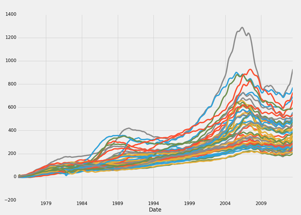
Bingo, that's what I am looking for! This is a % change for the HPI itself, by state. The first % change is still useful too for various reasons. We may wind up using that one in conjunction or instead, but, for now, we'll stick with typical % change from a starting point.

Now, we may want to bring in the other data sets, but let's see if we can get anywhere on our own. First, we could check some sort of "benchmark" so to speak. For this data, that benchmark would be the House Price Index for the United States. We can collect that with:

def HPI_Benchmark():
    df = Quandl.get("FMAC/HPI_USA", authtoken=api_key)
    df["United States"] = (df["United States"]-df["United States"][0]) / df["United States"][0] * 100.0
    return df

Then we'll do:

fig = plt.figure()
ax1 = plt.subplot2grid((1,1), (0,0))

HPI_data = pd.read_pickle('fiddy_states3.pickle')
benchmark = HPI_Benchmark()
HPI_data.plot(ax=ax1)
benchmark.plot(color='k',ax=ax1, linewidth=10)

plt.legend().remove()
plt.show()

Output:

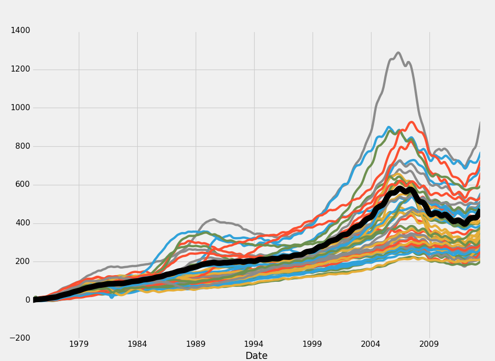
Looking at this data, it appears to be that all markets are relatively closely obeying each other as well as the overall house price index. There does exist some mean deviation here, but basically every market appears to follow a very similar trend. There winds up being quite a major divergence in the end, from 200% increase to over 800% increase, so obviously we have a major divergence there, but the mean is between 400 and 500% growth in the last upper 30 years.

How might we approach the markets possibly? Later on, we could take demographics and interest rates into consideration for predicting the future, but not everyone is interested in the game of speculation. Some people want more safe and secure investments instead. It looks to me here, like the housing markets just never really fail on a state-level. Obviously our plan might fail if we buy a home that later we find out has a major termite infestation and could collapse at any moment.

Staying macro, it is clear to me that we could engage in a very, apparently, safe pair-trading situation here. We can collect correlation and covariance information very easily with Pandas. Correlation and Covariance are two very similar topics, often confused. Correlation is not causation, and correlation is almost always included in covariance calculations for normalizing. Correlation is the measure of the degree by which two assets move in relation to eachother. Covariance is the measure of how two assets tend to vary together. Notice that correlation is a measure to the "degree" of. Covariance isn't. That's the important distinction if my own understanding is not incorrect!

Let's create a correlation table. What this will do for us, is look back historically, and measure the correlation between every single state's movements to every other state. Then, when two states that are normally very highly correlated start to diverge, we could consider selling property in the one that is rising, and buying property in the one that is falling as a sort of market neutral strategy where we're just profiting on the gap, rather than making some sort of attempt to predict the future. States that border each other probably are more likely to have more similar correlations than those far away, but we'll see what the numbers say.

HPI_data = pd.read_pickle('fiddy_states3.pickle')
HPI_State_Correlation = HPI_data.corr()
print(HPI_State_Correlation)

The output should be 50 rows x 50 columns, here's some of the output:

          AL        AK        AZ        AR        CA        CO        CT  \
AL  1.000000  0.944603  0.927361  0.994896  0.935970  0.979352  0.953724   
AK  0.944603  1.000000  0.893904  0.965830  0.900621  0.949834  0.896395   
AZ  0.927361  0.893904  1.000000  0.923786  0.973546  0.911422  0.917500   
AR  0.994896  0.965830  0.923786  1.000000  0.935364  0.985934  0.948341   
CA  0.935970  0.900621  0.973546  0.935364  1.000000  0.924982  0.956495   
CO  0.979352  0.949834  0.911422  0.985934  0.924982  1.000000  0.917129   
CT  0.953724  0.896395  0.917500  0.948341  0.956495  0.917129  1.000000   
DE  0.980566  0.939196  0.942273  0.975830  0.970232  0.949517  0.981177   
FL  0.918544  0.887891  0.994007  0.915989  0.987200  0.905126  0.926364   
GA  0.973562  0.880261  0.939715  0.960708  0.943928  0.959500  0.948500   
HI  0.946054  0.930520  0.902554  0.947022  0.937704  0.903461  0.938974   
ID  0.982868  0.944004  0.959193  0.977372  0.944342  0.960975  0.923099   
IL  0.984782  0.905512  0.947396  0.973761  0.963858  0.968552  0.955033   
IN  0.981189  0.889734  0.881542  0.973259  0.901154  0.971416  0.919696   
IA  0.985516  0.943740  0.894524  0.987919  0.914199  0.991455  0.913788   
KS  0.990774  0.957236  0.910948  0.995230  0.926872  0.994866  0.936523   
KY  0.994311  0.938125  0.900888  0.992903  0.923429  0.987097  0.941114   
LA  0.967232  0.990506  0.909534  0.982454  0.911742  0.972703  0.907456   
ME  0.972693  0.935850  0.923797  0.972573  0.965251  0.951917  0.989180   
MD  0.964917  0.943384  0.960836  0.964943  0.983677  0.940805  0.969170   
MA  0.966242  0.919842  0.921782  0.966962  0.962672  0.959294  0.986178   
MI  0.891205  0.745697  0.848602  0.873314  0.861772  0.900040  0.843032   
MN  0.971967  0.926352  0.952359  0.972338  0.970661  0.983120  0.945521   
MS  0.996089  0.962494  0.927354  0.997443  0.932752  0.985298  0.945831   
MO  0.992706  0.933201  0.938680  0.989672  0.955317  0.985194  0.961364   
MT  0.977030  0.976840  0.916000  0.983822  0.923950  0.971516  0.917663   
NE  0.988030  0.941229  0.896688  0.990868  0.912736  0.992179  0.920409   
NV  0.858538  0.785404  0.965617  0.846968  0.948143  0.837757  0.866554   
NH  0.953366  0.907236  0.932992  0.952882  0.969574  0.941555  0.990066   
NJ  0.968837  0.934392  0.943698  0.967477  0.975258  0.944460  0.989845   
NM  0.992118  0.967777  0.934744  0.993195  0.934720  0.968001  0.946073   
NY  0.973984  0.940310  0.921126  0.973972  0.959543  0.949474  0.989576   
NC  0.998383  0.934841  0.915403  0.991863  0.928632  0.977069  0.956074   
ND  0.936510  0.973971  0.840705  0.957838  0.867096  0.942225  0.882938   
OH  0.966598  0.855223  0.883396  0.954128  0.901842  0.957527  0.911510   
OK  0.944903  0.984550  0.881332  0.967316  0.882199  0.960694  0.879854   
OR  0.981180  0.948190  0.949089  0.978144  0.944542  0.971110  0.916942   
PA  0.985357  0.946184  0.915914  0.983651  0.950621  0.956316  0.975324   
RI  0.950261  0.897159  0.943350  0.945984  0.984298  0.926362  0.988351   
SC  0.998603  0.945949  0.929591  0.994117  0.942524  0.980911  0.959591   
SD  0.983878  0.966573  0.889405  0.990832  0.911188  0.984463  0.924295   
TN  0.998285  0.946858  0.919056  0.995949  0.931616  0.983089  0.953009   
TX  0.963876  0.983235  0.892276  0.981413  0.902571  0.970795  0.919415   
UT  0.983987  0.951873  0.926676  0.982867  0.909573  0.974909  0.900908   
VT  0.975210  0.952370  0.909242  0.977904  0.949225  0.951388  0.973716   
VA  0.972236  0.956925  0.950839  0.975683  0.977028  0.954801  0.970366   
WA  0.988253  0.948562  0.950262  0.982877  0.956434  0.968816  0.941987   
WV  0.984364  0.964846  0.907797  0.990264  0.924300  0.979467  0.925198   
WI  0.990190  0.930548  0.927619  0.985818  0.943768  0.987609  0.936340   
WY  0.944600  0.983109  0.892255  0.960336  0.897551  0.950113  0.880035  

So now we can see correlation in HPI movements between every single state pair. Very interesting, and, as is glaringly obvious, all of these are pretty high. Correlation is bounded from -1 to positive 1. 1 being a perfect correlation, and -1 being a perfect negative correlation. Covariance has no bound. Wonder about some more stats? Pandas has a very nifty describe method:

print(HPI_State_Correlation.describe())

Output:

              AL         AK         AZ         AR         CA         CO  \
count  50.000000  50.000000  50.000000  50.000000  50.000000  50.000000   
mean    0.969114   0.932978   0.922772   0.969600   0.938254   0.958432   
std     0.028069   0.046225   0.031469   0.029532   0.031033   0.030502   
min     0.858538   0.745697   0.840705   0.846968   0.861772   0.837757   
25%     0.956262   0.921470   0.903865   0.961767   0.916507   0.949485   
50%     0.976120   0.943562   0.922784   0.976601   0.940114   0.964488   
75%     0.987401   0.957159   0.943081   0.989234   0.961890   0.980550   
max     1.000000   1.000000   1.000000   1.000000   1.000000   1.000000   

              CT         DE         FL         GA    ...             SD  \
count  50.000000  50.000000  50.000000  50.000000    ...      50.000000   
mean    0.938752   0.963892   0.920650   0.945985    ...       0.959275   
std     0.035402   0.028814   0.035204   0.030631    ...       0.039076   
min     0.843032   0.846668   0.833816   0.849962    ...       0.794846   
25%     0.917541   0.950417   0.899680   0.934875    ...       0.952632   
50%     0.941550   0.970461   0.918904   0.949980    ...       0.972660   
75%     0.960920   0.980587   0.944646   0.964282    ...       0.982252   
max     1.000000   1.000000   1.000000   1.000000    ...       1.000000   

              TN         TX         UT         VT         VA         WA  \
count  50.000000  50.000000  50.000000  50.000000  50.000000  50.000000   
mean    0.968373   0.944410   0.953990   0.959094   0.963491   0.966678   
std     0.029649   0.039712   0.033818   0.035041   0.029047   0.025752   
min     0.845672   0.791177   0.841324   0.817081   0.828781   0.862245   
25%     0.955844   0.931489   0.936264   0.952458   0.955986   0.954070   
50%     0.976294   0.953301   0.956764   0.968237   0.970380   0.974049   
75%     0.987843   0.967444   0.979966   0.976644   0.976169   0.983541   
max     1.000000   1.000000   1.000000   1.000000   1.000000   1.000000   

              WV         WI         WY  
count  50.000000  50.000000  50.000000  
mean    0.961813   0.965621   0.932232  
std     0.035339   0.026125   0.048678  
min     0.820529   0.874777   0.741663  
25%     0.957074   0.950046   0.915386  
50%     0.974099   0.973141   0.943979  
75%     0.984067   0.986954   0.961900  
max     1.000000   1.000000   1.000000  

[8 rows x 50 columns]

This tells us, per state, what the lowest correlation was, what the average correlation was, what the standard deviation is, the 25% lowest, the middle (median / 50%)... and so on. Obviously they all have a max 1.0, because they are perfectly correlated with themselves. Most importantly, however, all of these states that we're seeing here (some of the 50 columns are skipped, we go from GA to SD) have above a 90% correlation with everyone else on average. Wyoming gets as low as 74% correlation with a state, which, after looking at our table, is Michigan. Because of this, we would probably not want to Invest in Wyoming, if Michigan is leading the pack up, or sell our house in Michigan just because Wyoming is falling hard.

Not only could we look for any deviations from the overall index, we could also look for deviations from the individual markets as well. As you can see, we have the standard deviation numbers for every state. We could make attempts to invest in real estate when the market falls below the standard deviations, or sell when markets get above standard deviation. Before we get there, let's address the concepts of smoothing out data, as well as resampling, in the next tutorial.

The next tutorial: Resampling - p.9 Data Analysis with Python and Pandas Tutorial